Over the years in the audio industry, I have made numerous attempts to explain some of the concepts used with regard to speaker/amplifier power. Most are summarised below, with links to some of the articles covering each topic in more detail. If you’re serious about sound, and curious about power, these are well worth a read, and will help you make more sense of power.
What is Power (Watts)?
Power is a measure of how fast energy is being used or delivered. One watt is defined as one joule per second, which in audio terms is the rate at which energy is transferred from an amplifier to a loudspeaker. High power for a short burst and lower power delivered continuously can result in the same total energy, which is why power must be considered over time.
For example, a 4 W burst for 0.25 seconds followed by 0.75 seconds of silence delivers the same energy as a 2 W burst for 0.5 seconds followed by 0.5 seconds of silence, or 1 W delivered continuously for 1 second.
This simplified example is an analogy for understanding peak, program, and continuous power. Peak power represents short, high-energy bursts, program power represents longer bursts with more time at a high level, and continuous power represents energy delivered without breaks. Although real music does not follow fixed duty cycles, all three cases above average to the same energy rate: 4 W × 0.25 = 1, 2 W × 0.5 = 1, and 1 W × 1 = 1.
This is why loudspeaker power ratings typically follow the same pattern: program power is usually twice the continuous rating, and peak power is typically four times the continuous rating. The numbers relate to the same underlying energy, but describe how that power is delivered over time.
RMS Power
RMS is a mathematical method that works extremely well for steady sine waves, such as AC mains power, where voltage and current are continuous and predictable. Music is not like this, so “RMS power” is not ideal for describing real audio behaviour. Some amplifier manufacturers still use the term, but it often includes a hidden crest factor or burst condition, meaning the figure is not a true continuous power level but a calculated equivalent. Read more…
AES / Continuous Power
AES power defines how much power a loudspeaker can handle on average over time using a standardised broadband noise signal. It represents the long-term thermal limit of the voice coil and is the most reliable figure for continuous operation. Unlike RMS-style ratings, AES power is designed specifically for real audio signals rather than steady test tones.
Program (Music) Power
Program power allows for higher short-term peaks while keeping the long-term average power the same as the AES rating. It reflects the dynamic nature of music, where loud transients are followed by quieter moments. Program power is headroom, not extra continuous power, and should never be treated as a sustained operating level. Read More on AES / Program Power
How much Power do you need?
What’s up with the Watts?
Power ratings in audio can be confusing because music is dynamic, not constant. Its hard to know what you want, what’s best and how to use power figures sensibly when choosing speakers and amplifiers. Read More…
Pe – Power Handling Capacity
Often seen in manufacturers technical data, Pe is the long term power handling capacity, usually measured using the AES standard (but not always) and some manufacturers have their own test criteria and will often name this ‘nominal power handling’ This is not necessarily comparable between all speaker brands – also a little explanation as to why MORE POWER does not necessarily mean MORE VOLUME Read More..
RMS stands for Root Mean Square. It is a mathematical method, not a type of power. It is normally applied to voltage or current, but for many years it has been used in the audio industry to describe amplifier and loudspeaker power.
Why? Simply because it was the best available method at the time, and no better, widely agreed standard existed.
I am often asked “What’s the RMS power?” My usual answer is that RMS is not particularly suitable for audio. If you want to understand why, read on. Otherwise, just accept that AES power is the standard you should be using for loudspeakers.
Why do we have RMS at all?
RMS comes from electrical engineering, where it works extremely well for AC power systems. It allows an AC signal to be converted into an equivalent DC value that produces the same heating effect.
In the UK, mains electricity is described as 240 V AC. That figure is already an RMS value. In reality, the waveform swings to about 339 V peak, or 679 V peak-to-peak.
The RMS figure is very useful. If an electric heater draws 10 A from a 240 V supply, we call it a 2400 W heater. The voltage and current are constant, the waveform is a steady 50 Hz sine wave, and the power delivery is continuous. This is a perfect use case for RMS.
[Image: AC sine wave showing peak, peak-to-peak, and RMS level]
Why RMS doesn’t map cleanly to audio
Audio amplifiers and loudspeakers do not operate with constant sine waves. Music is dynamic, the amplitude changes constantly, and power delivery is anything but steady.
To work around this, various test standards were created using controlled noise signals instead of tones. For loudspeakers, common examples included EIA RS-426A and IEC 268-5.
With a known test signal, it is possible to calculate an equivalent RMS value using averaging and squaring maths. This is where the idea of “RMS power” for speakers came from. However, it was never especially accurate, and often resulted in unrealistically low power ratings.
The amplifier vs speaker mismatch
Over time, it became normal to match amplifier and speaker ratings directly. For example, using a 400 W RMS amplifier with a 400 W RMS speaker.
The problem is that the two numbers were not measuring the same thing.
Amplifiers were often tested at 1 kHz using a continuous sine wave into a resistive load. This frequently overstated real-world power, because at lower frequencies (around 40–100 Hz) the power supply could not always sustain the same output. In practice, usable power at 100 Hz could be 10% lower than at 1 kHz.
Meanwhile, loudspeakers could often tolerate short-term peaks above their RMS rating. This is why users traditionally chose a slightly larger amplifier, to provide headroom.
Conclusion
RMS was not useless, but it was never a complete or accurate way to relate amplifier power to loudspeaker power. There was always an element of estimation and experience involved.
This mismatch is exactly why modern standards moved on, and why RMS power is no longer the best reference point for real-world audio systems.
AES Power, Program Power, and Amplifier Power Explained
Power ratings in audio are confusing because they try to describe something that is constantly changing. Music is not a steady signal, yet power ratings are often presented as if everything operates at a fixed level. To make sense of AES power, program power, and amplifier power ratings, it helps to think in terms of power over time, rather than a single number.
Summary
AES power describes how much power a loudspeaker can handle on average over time. Program (music) power allows for higher short-term peaks, not higher continuous power. Real music delivers power in bursts rather than as a constant load. Modern amplifiers, especially Class D designs, are very good at producing high peak power briefly, while long-term power is limited by heat, power supplies, and mains capacity. The aim of this article is to show how average power, burst power, and time are related, and why a headline figure such as a 2000 W peak can be entirely real while still not representing the long-term power demand of a system. By looking at how music behaves over time, and using simple visual examples, it becomes much easier to understand how loudspeaker ratings, amplifier ratings, and even 13 A mains plugs all make sense in practice.
AES Power vs Program (Music) Power
Modern loudspeaker drivers are usually specified with two related power figures: continuous power (often defined using the AES standard) and program or music power.
AES power represents the long-term average thermal capability of the loudspeaker. It indicates how much power the voice coil can safely dissipate as heat over time using a defined broadband test signal. In simple terms, AES power is a safe long-term operating limit.
Program (music) power is typically quoted as twice the AES power, which corresponds to a +3 dB increase. Importantly, this does not mean the loudspeaker can handle twice the average power. The long-term average power remains the same as the AES rating.
The difference between AES and program power is not extra heat capacity, but crest factor. Program power allows for higher short-term peaks while keeping the long-term average unchanged. The signal is allowed to get taller for brief moments, but not heavier overall.
To understand why this distinction matters, it helps to look at how power is delivered over time.
Power over time: short, high peaks
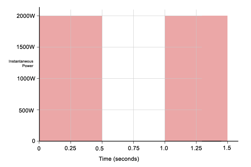
In the first diagram, the vertical axis represents instantaneous power, and the horizontal axis represents time. The shaded red areas show when power is being delivered.
The diagrams are illustrative rather than literal. Their purpose is to explain concepts, not to define exact test conditions or limits.
Figure 1: Short-duration, high-peak power delivered in brief bursts over time.
Each rectangle represents a short burst of power:
Peak power: 2000 W
Duration: 0.5 seconds
Power multiplied by time gives energy. A 2000 W burst lasting 0.5 seconds delivers the same energy as 1000 W delivered for a full second:
2000 W × 0.5 s = 1000 W × 1 s
Although the instantaneous power is high, it is only present briefly. When averaged over a longer time window, the effective power is much lower. This is the key idea behind program power: higher peaks are allowed, but they do not increase the long-term average.
This type of power delivery closely resembles real music. Bass hits, kick drums, and transients are short, intense bursts separated by quieter moments.
To make the diagrams easier to understand, I have intentionally used simple numbers, 2000W, 1000W, 0.5 seconds – it makes the maths much easier. You can see each red rectangle is divided up into 8 smaller rectangles, which is easy to visualise.
Same energy, delivered differently
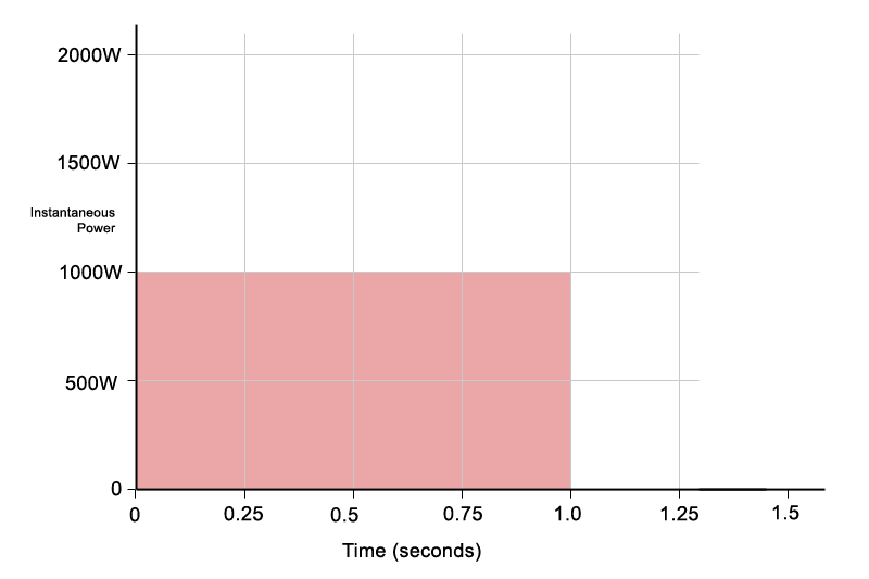
In the Figure 2, the same total energy is delivered in a different way. Instead of short peaks, power is delivered continuously. This is similar to electrical systems such as heaters, power is delivered continuously to a static load, the power level does not go up or down, it remains constant. Music is not like this, amplifier and music power is dynamic, and constantly changing. The power an amplifier delivers to the speaker, and draws from the mains supply varies with time.
Figure 2: The same total energy delivered as lower, continuous power over the same time period.
Power level: 1000 W
Duration: 1 second
The shaded area is the same size as in the Figure 1, which means the total energy is identical. The average power is also the same. You can see this visually: the area still covers exactly eight grid squares, just arranged differently.
In this example, the continuous 1000 W case does not represent a significant challenge for the amplifier. An amplifier capable of delivering 2000 W peaks will typically have no difficulty sustaining 1000 W continuously, as the average power and thermal load remain well within its design limits.
The real limitation appears when high power is sustained for longer periods. While short bursts of 2000 W are easily achievable, maintaining that level for several seconds places extreme demands on the power supply and output stage. Voltage rails sag, current limiting engages, and thermal protection may begin to operate.
This is where many Class D amplifiers reach their limits. They are designed to deliver very high short-term power with ease, but they are not intended to sustain maximum output continuously, particularly at low frequencies.
What this means for loudspeakers
From the loudspeaker’s point of view, heating depends on average power over time, not peak power. The voice coil does not care whether energy arrives in short bursts or steadily; what matters is how much heat builds up overall.
AES power therefore describes a realistic long-term thermal limit. It represents the average power a loudspeaker can dissipate safely over time without overheating. In the simplified examples shown here, this is illustrated by the second diagram, where the average power level remains constant.
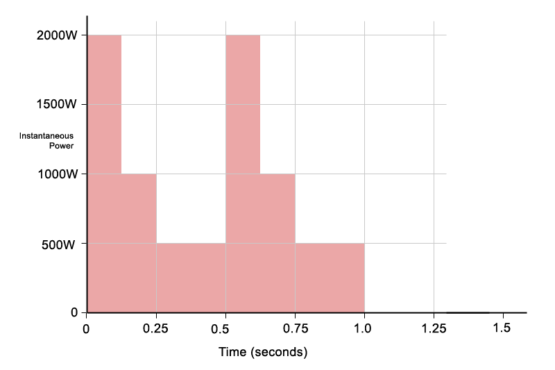
Program or music power acknowledges that real music is dynamic and contains peaks and lulls. This is illustrated in the Figure 3, where the total shaded area remains the same, but the instantaneous power rises to higher peaks. The average power is unchanged, the program material just has a higher crest factor with more pronounced peaks and lulls.
Figure 3: Illustrating crest factor for music/program power.
This simplified example shows how a loudspeaker can safely handle higher short-term peaks, provided the long-term average power remains within the AES rating. Program power just shows the speaker can handle higher short term peaks, as long as the long-term average power remains within the AES limit.
Problems arise when program power is treated as a continuous operating level. If the programme material has little dynamic range, or if heavy compression and limiting are applied, the crest factor is reduced and the average power rises toward the peak level. In this situation the loudspeaker is no longer operating within its intended thermal limits and the voice coil can overheat.
Program power is therefore best understood as a headroom allowance for dynamic signals, not as a sustained power rating. It best represents live music, particularly percussive sounds. Electronic, synthesised music is often compressed, and has long extended bass notes with low dynamics.
What this means for amplifiers
Modern amplifiers, particularly Class D designs, behave much like the first diagram rather than the second.
They are extremely good at delivering short bursts of high power thanks to high-voltage rails and efficient output stages. This is why many modern amplifiers are rated using standards such as EIAJ, which better reflect burst capability and musical crest factor.
What these amplifiers cannot do is sustain very high power indefinitely, especially at low frequencies. Long, continuous bass notes place heavy demands on the power supply, causing voltage sag, current limiting, or thermal protection to intervene.
This is why amplifier power ratings often look impressive on paper but drop significantly under continuous sine-wave testing, particularly into low impedances.
Matching amplifier power to speaker power
Program power is useful when choosing an amplifier because it indicates how much headroom is available for musical peaks. A common and sensible approach is to choose an amplifier capable of delivering somewhere between the AES power and the program power of the loudspeaker.
This provides enough headroom for dynamics without pushing the driver beyond its long-term thermal limits. However, once amplifier power approaches program ratings, proper use of limiters and compressors becomes essential to prevent excessive average power.
How can this make sense on a 13A plug?
The same power-over-time logic also explains why large amplifiers can operate from ordinary mains supplies. To take this one step further, it is useful to look at a more realistic musical signal rather than a simple rectangle, which represents power being fully on or fully off.
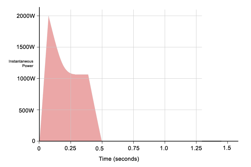
Figure 4 shows a simplified ADSR-style envelope, loosely resembling a typical percussive sound such as a drum hit. The instantaneous power still rises briefly to around 2000 W, but the time spent at high power is much shorter than in the rectangular examples.
Figure 4: A simplified percussive envelope showing brief high-power peak typical of a real musical signal.
As a result, the total shaded area is smaller, meaning less total energy is delivered overall. Despite the high peak, the average power remains relatively low. This is exactly the type of signal that modern Class D amplifiers handle extremely well: short, high-power bursts delivered cleanly without clipping and distortion. To clarify, this is not intended to suggest that a Class D amplifier cannot sustain peaks for longer than shown – indeed most can. The diagram is simply a representative example of real-world music, intended to show how musical signals translate into long-term average power, and why the ability to handle short bursts of high power is important for preserving dynamics.
This behaviour explains why large amplifiers can produce impressive peak power figures while still operating safely from standard mains connections. The peaks are brief, the average power is modest, and the electrical system only needs to support the long-term average rather than the instantaneous maximum.
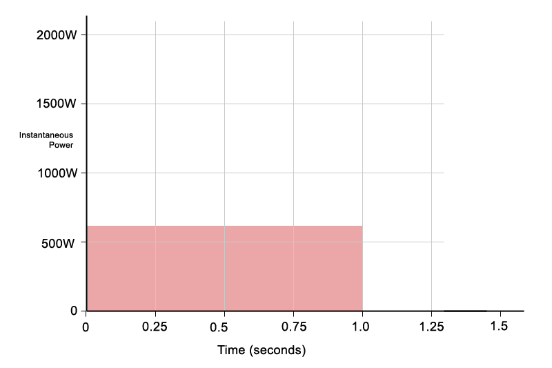
For reference, the percussive example above has been approximated into a final diagram (Fig. 5) showing the same energy spread out as continuous power over time. Although the instantaneous peak reaches around 2000 W very briefly, the equivalent long-term average power is much lower, in the region of 600W.
Figure 5: The same energy from Figure 4 redistributed as continuous power, showing the equivalent long-term average.
This illustrates an important point: a short, high-power percussive event may look extreme when viewed instantaneously, but when averaged over time it represents a far more modest power demand. Even when additional sounds are present, the medium-term average power may only rise to around 800-900 W.
Applied across a four-channel amplifier, this suggests that even when all channels are working hard, the combined long-term average power is often closer to 3000W rather than the headline peak figures. While this approaches the practical limits of a 13 A mains supply, real music contains loud passages, quieter sections, and natural breaks. These variations reduce the long-term average further, keeping operation within safe limits.
This is why high-power amplifiers can operate from standard mains connections. Peak power figures describe short-term capability, not continuous demand. In the case of amplifiers such as the JAM Systems Q10, which is rated at up to 2500 W EIAJ per channel into 2 ohms, the apparent mismatch between output power and a 13 A plug disappears once power is considered over time rather than at its instantaneous maximum. Realistically this amp is at the limits of a 13A supply, which is why it comes with a heavy duty mains cable with 2.5mm cable and a heavy duty plug.
After being asked countless times how the JAM Systems Q10 can operate from a 13A plug, this article was written to explain exactly that. This article now serves as the standard explanation.
The key takeaway
Power ratings make far more sense when you consider how power is delivered over time. Peak power, program power, and amplifier ratings all describe different aspects of the same thing: short-term capability versus long-term limits.
Many people dismiss peak power figures because of how terms such as PMPO were misused in consumer hi-fi, often wildly overstating real capability. However, genuine high burst power serves a real purpose. It allows the dynamics of the original programme material to be preserved, delivering very large transients when required, but only for short periods of time.
AES power defines what is safe on average. Program power defines how much headroom is available for musical peaks. Understanding the difference makes amplifier choice, system setup, and real-world behaviour far easier to predict.
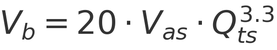
The full formula for calculating ‘optimum box volume’ is:
Vas, Qts and fs are all known numbers, and are available from the TS Parameters published for the speaker driver you want to use. However to use the above formula, you need to determine fb which is the tuning frequency of the ports in the cabinet. Its generally considered that you get the best results by selecting a tuning frequency just slightly higher than fs – it gives the best combination of performance improvements. The aim of the ported cabinet is to extend the bass response, and enhance the lower bass output, getting the right cabinet volume and correct fb also helps maintain damping and give a smoother bass roll off, whilst at the same time controlling excursion at bass frequencies to prevent over-excursion. If you’ve read about fs you’ll already know this is the frequency that the woofer naturally moves easiest, if it moves too much, it will get damaged. The ports reduce the cone excursion around fb so its sensible to keep this near fs to keep the overall cone excursion under control.
At this stage we are just trying to work out an approximate target volume for the cabinet based on the desired tuning frequency. The final tuning frequency of the box, fb is determined by the port dimensions and length with respect to the box volume. We are not setting fb with the box volume, we’re just estimating a target box volume that’s suitable for the driver to get good results.
The above formula would prove useful if you are aiming to get a small compact cabinet with optimum damping, but sacrificing bass extension. If you have enough headroom to compensate with DSP, this would allow for some very compact designs, particularly if punchy bass is the target.
Assuming we are looking to achieve good bass extension, common in large format PA applications, it would be simpler to just use fs = fb to get a typical cabinet volume, this simplifies the equation to:
Our recommendation is that this would normally be a good target volume for good bass response, and you could adjust this according to your design objective. You don’t want to make it too large, as this will compromise damping, so perhaps up to 30% larger for deep bass. If you want a compact cabinet, 10%-15% smaller if you are willing to have some compromise on bass extension to minimise cabinet volume.
Here are some example calculations for a popular 18″ woofer:
Vas = 212 litres
Qts = 0.35
fs = 34 Hz
Vb = 20 × 212 × (0.35)3.3 ≈ 132.7 litres
This gives a practical starting point for designing a PA bass reflex enclosure. It aligns closely with real-world cabinet sizes — allowing for bracing, port volume, and tuning flexibility — while remaining efficient and well-controlled for live sound applications. Remember this is the REMAINING volume after subtracting handles, ports, braces, and the volume of the driver itself. Your unloaded cabinet would probably need to be around 150 litres when designed.
To make the most compact cabinet, you could reduce this to 125 litres, and accept reduced low frequency extension, but potentially the ability to tune for tight punchy bass above fs
If you want more deep bass, and size isn’t an issue, a 200 litre cabinet would give more options for lower tuning, deeper bass, but most likely worse damping (sloppy or less responsive bass) and lower efficiency.
So you can see, cabinet volume can vary a lot, the driver will still work, but the results will also vary.
When designing a speaker enclosure, especially a ported (bass reflex) box, it’s a common misconception that there’s one perfect cabinet volume for every driver. In reality, there’s a range of suitable volumes, each delivering a slightly different result depending on the design goal. Cabinet volume has a direct effect on bass response — not just in terms of depth, but in how the bass feels: tight and punchy vs deep and smooth.
The internal volume of the box interacts with the driver’s compliance (represented by Vas) and contributes to how freely the cone can move. A very large enclosure provides less air resistance (acoustic spring), allowing the cone to move more easily, which can improve low-end extension but may reduce control. Conversely, a smaller enclosure increases acoustic stiffness, restricting cone movement — which can tighten response but raise the system’s resonance.
It’s worth noting that modest changes in box volume aren’t inherently problematic. There’s no need to obsess over a perfect number — cabinet volume isn’t a razor-sharp target, but more of a zone you want to stay within. Problems tend to occur only when the volume is way off — such as using a box far too small or unnecessarily large for the driver. In practice, modern speaker designs aim for the smallest box possible that still delivers strong bass extension, reflecting a shift toward compact but efficient systems.
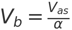
There’s always a trade-off between bass extension (how low it goes) and bass response (how tight or efficient it sounds). With that in mind, here’s a quick and practical method to estimate your starting box volume for a ported speaker:
Vb: Recommended internal cabinet volume (in litres)
Vas: Equivalent compliance volume of the driver (litres)
α: Alignment factor, typically between 1.5 and 3
What Does Alpha Mean?
The value of α (alpha) determines how large or small your cabinet will be, and how the bass response is shaped the value of α in the formula above is a scaling factor that reflects how the compliance of the air inside the box compares to the compliance of the driver’s suspension (Vas). The speaker cone and the air inside the cabinet form a mass-spring system, and the box volume determines how stiff the air spring is.
α ≈ 1.5 – A softer air spring, leading to a larger box. The cone moves more freely, resulting in better low-frequency extension. It’s close to a maximally flat alignment (like QB3 or SBB4), but physically bigger than most other options.
α ≈ 3 – A stiffer air spring, giving a smaller box. This restricts cone movement more, often creating a bass hump and a stronger punch in the upper bass, at the cost of earlier low-end roll-off. It’s closer to alignments like SC4 or EBS, often used for compact or punchy systems. It’s closer to alignments like SC4 or EBS, often used for compact or punchy systems.
Choosing your α value is about balancing size and performance. Lower values favour flat, extended bass; higher values prioritise compact design and punchy response. We recommend sticking between 1.5 and 3 for purposes of calculating ball park figures. Choosing α is essentially choosing your compromise: deep and flat but large vs compact and punchy, with less deep bass.
Example
Say your driver has:
Vas = 100 L
Qts = 0.35
This driver suits a range of box volumes depending on your design goals:
Flatter, deeper bass: Vb = 100 / 1.5 = 66.7 L
Compact, punchy box: Vb = 100 / 3 = 33.3 L
So your practical range is between 33 to 67 litres — smaller if you prioritise space, larger if you want extended bass depth.
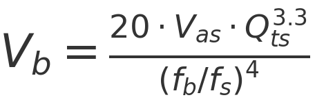
Please note, the above is a SIMPLIFIED calculator to estimate suitable cabinet sizes without getting too involved in the science. Here is the full formula:
This gives a more precise prediction based on Thiele-Small parameters and your chosen tuning frequency. Let’s break down what each part means:
Vb: Recommended internal box volume (litres)
Vas: Equivalent compliance volume of the driver (litres)
Qts: Total Q of the driver (combined electrical and mechanical losses)
fb: Desired box tuning frequency (Hz)
fs: Driver’s free-air resonance frequency (Hz)
What It Tells You
Higher Qts values usually call for a larger enclosure
Lower tuning frequencies (fb) increase the required volume
This formula is useful as a starting point for simulation tools. It’s more accurate than the simplified Vas/α method, but assumes a traditional alignment without DSP-based adjustments to compensate for bass response. It also allows you to specify your target tuning frequency. You should also note that Qts is quite significant in determining suitability for bass reflex enclosures. The useable range for Qts is typically 0.28 – 0.45 with a ‘sweet spot’ at 0.37-0.38 which tends to gives many of the best ‘all round general purpose’ woofers for ported enclosures. The above calculations will give you Vb results for Qts values outside of this range, but these will most likely result in poor performance, or give unrealistic volumes that are too large or too small.
We’re still updating and improving these pages, they are intended as general guidelines to help with the understanding of T&S Parameters and their relevance to speaker design. In some cases, a simplified explanation or example is used to illustrate a point, and may not be 100% accurate in all circumstances.,
BL (force factor) represents the strength of the magnetic motor system in a loudspeaker. It is calculated as the product of magnetic flux density (B) and length of wire in the magnetic field (L), measured in Tesla meters (T·m). A higher BL indicates a stronger motor, which generally improves control over the cone.
Mms refers to the total mass of all moving components of the driver, including the cone, voice coil, dust cap, and the air load around the diaphragm. A higher Mms generally results in a lower resonant frequency (Fs), which can help extend bass response, but it also requires more energy to move. Conversely, a lower Mms allows for better transient response, making it ideal for midrange drivers.
Cms – Compliance of the Driver Suspension> read more
Cms represents the compliance of a speaker’s suspension system, essentially measuring its flexibility. It’s the inverse of stiffness; a higher Cms indicates a more pliable suspension, allowing the cone to move more freely. This flexibility affects the driver’s resonant frequency (Fs); a more compliant suspension results in a lower Fs, enabling better low-frequency reproduction.
Rms – Mechanical Resistance of the Suspension> read more
Rms denotes the mechanical resistance within the driver’s suspension, quantifying the inherent damping due to the materials and construction of components like the surround and spider. Higher Rms values indicate greater energy loss, which can dampen cone movement and affect the driver’s transient response. Balancing Rms is crucial for achieving desired sound characteristics, as excessive mechanical resistance can lead to reduced efficiency and dynamic range.
Sd refers to the effective surface area of the driver’s diaphragm (cone) that actively moves air. It’s typically measured in square meters (m²). A larger Sd allows the driver to displace more air, contributing to higher sound pressure levels, especially at low frequencies. Accurately determining Sd involves measuring the cone’s diameter and accounting for the surround’s contribution to the moving area.
η₀ represents the efficiency of the driver, given as a percentage, showing how well it converts electrical power into acoustic output. A higher η₀ means the driver is more efficient and produces more SPL for the same input power. Efficiency is closely related to BL, Sd, and Mms, with high-efficiency drivers typically having a strong motor (high BL) and lightweight moving parts (low Mms).
Fs is the frequency at which the driver naturally resonates when not mounted in an enclosure. It is determined by the moving mass (Mms) and compliance (Cms) of the driver. Lower Fs values indicate better suitability for subwoofers, while higher Fs values are typical for midrange and tweeters, where tight cone control is needed.
Z is the nominal impedance of the driver, typically 4Ω, 8Ω, or 16Ω, and represents the average electrical resistance presented to an amplifier. While Re (DC resistance) is slightly lower, the impedance of a driver varies across different frequencies due to Le (voice coil inductance) and resonance effects.
Vas represents the volume of air that exhibits the same compliance as the driver’s suspension. Measured in liters, it provides insight into how the driver interacts with the air in an enclosure. A larger Vas suggests a more compliant suspension, often necessitating a larger enclosure for optimal performance. Understanding Vas aids in designing speaker cabinets that complement the driver’s mechanical properties.
Pe indicates the thermal power handling capacity of the driver, measured in watts. It defines the maximum continuous power the driver can handle without incurring thermal damage to components like the voice coil. Exceeding Pe can lead to overheating and potential failure. It’s essential to match the amplifier’s output with the driver’s Pe to ensure reliability and longevity.
Xmax defines the maximum distance the driver’s cone can move linearly in one direction without significant distortion. Measured in millimeters, it reflects the limits of the voice coil’s travel within the magnetic gap. Exceeding Xmax can cause nonlinear behavior, leading to distortion and potential mechanical damage. Designing with an appropriate Xmax ensures the driver can handle desired sound pressure levels without compromising sound quality.
Xlim – Maximum Physical Excursion Before Damage > read more
Xlim, also known as Xmech or Xdamage, specifies the absolute maximum excursion the driver can endure before mechanical failure occurs. Surpassing Xlim can result in physical damage to components such as the voice coil, spider, or surround. It’s crucial to ensure that the driver operates within safe excursion limits, especially in high-power applications, to maintain durability and performance.
Le measures the inductance of the voice coil, typically in millihenries (mH). This parameter affects the driver’s impedance at higher frequencies, influencing the crossover design and overall frequency response. A higher Le can lead to a roll-off in the high-frequency response, making it essential to consider in the design of midrange and high-frequency drivers.
Re denotes the direct current (DC) resistance of the voice coil, measured in ohms (Ω). It’s a fundamental parameter that influences the driver’s electrical damping (Qes) and overall impedance. Accurate knowledge of Re is vital for matching the driver with the amplifier and designing appropriate crossover networks.
Qes represents the electrical damping of the driver at its resonant frequency (Fs). It reflects how the driver’s electrical characteristics control its resonance. A lower Qes indicates higher electrical damping, leading to tighter control over cone movement, which is desirable in achieving accurate sound reproduction.
Qms quantifies the mechanical damping of the driver, considering losses in the suspension system. It indicates how the mechanical properties influence the driver’s resonance. A higher Qms suggests lower mechanical losses, resulting in a more resonant system. Balancing Qms with Qes is essential for achieving the desired total damping (Qts) and overall sound quality.
Qtsis the combined quality factor that accounts for both electrical (Qes) and mechanical (Qms) damping. It provides a comprehensive understanding of the driver’s damping characteristics at resonance. The value of Qts influences enclosure design decisions:
Vd is the product of the effective diaphragm area (Sd) and the maximum linear excursion (Xmax). It quantifies the maximum volume of air the driver can displace, directly influencing its ability to produce low-frequency sound. A higher Vd indicates greater potential for bass output, making it a useful parameter when selecting a suitable woofer.
EBP (Efficiency Bandwidth Product) is a quick way to estimate whether a driver is better suited for a sealed or ported enclosure, calculated as Fs / Qes. A low EBP (< 50) suggests the driver works best in sealed enclosures, while a high EBP (> 100) indicates it is more suitable for ported or horn-loaded designs. While useful as a guideline, EBP isn’t an absolute rule—other factors like Vas, Xmax, and BL also influence enclosure choice.
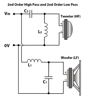
If you’ve been researching online about crossover design and tried inputting values into a crossover calculator, you might believe that you’re prepared to dive into the realm of professional audio. You might feel ready to embark on designing your own speakers and crossovers. However, once you start the actual process, you’ll quickly realize that theory and reality exist in separate realms, particularly true when it comes to passive crossovers and speakers.
So, what’s the challenge? The primary hurdle stems from the fact that nearly all online crossover calculators, textbooks, and the typical approach taken by beginners in crossover design make the assumption that both the Woofer and Tweeter possess an impedance of 8 ohms. Moreover, this assumed impedance remains constant across all frequencies, and their frequency responses are both flat and balanced. However, this is where reality intervenes. Once you begin examining the impedance measurements and frequency responses of the actual components you intend to use, the issues become readily apparent.
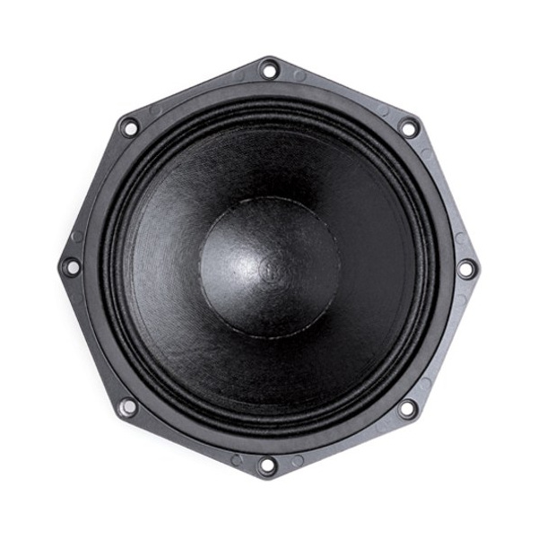
For our illustrative project, we’ve opted to work with a well-known 8″ PA Woofer: the B&C 8NDL51. Analyzing the graph below, we can observe that the impedance sits at 8 ohms around 800Hz. Consequently, at this frequency, our theoretical crossover derived from an online calculator should perform as expected in the real world.
However, our goal is not to establish a crossover point at 800Hz. In order to align with a smaller tweeter, we aim for a crossover frequency around 2500Hz or slightly higher. At the 2500Hz mark, the woofer’s impedance measures around 11 ohms and continues to rise beyond this point. If we were to input 11 ohms instead of 8 ohms into a crossover calculator, we might achieve a more favorable outcome. Nevertheless, due to the fluctuating impedance, predicting the results becomes challenging, making it difficult to determine the optimal choice.
If the objective is to stabilize the impedance load of the woofer, there are potential solutions available. However, these solutions can become intricate and potentially costly. Delving into the intricate details of crafting the ideal crossover leads us to the realm of Zobel Networks. While we occasionally employ Zobel networks, our focus primarily centers on crafting uncomplicated crossover designs that remain cost-effective to produce.
When it comes to crossover design, we start by examining the impedance and frequency responses. This analysis aids us in determining the best approach. We have already measured impedance, our next task is to measure the frequency response. This step assists us in selecting a starting filter frequency. However, it’s common for us to experiment with various filter configurations before pinpointing the one that works the best.
The frequency response measurements have all been conducted utilizing a clio system paired with an appropriate microphone. As these measurements predominantly serve the purpose of illustrating comparative outcomes for educational intents, we haven’t taken the effort to meticulously calibrate the settings to precisely 1W/1M. The measurements were taken within a standard room, where minimal sound-absorbing materials have been strategically positioned on the walls to curtail reflections. It’s important to note that all the measurements presented below capture room reflections and anomalies induced by the environment. Consequently, they don’t offer a true representation of the exact response.
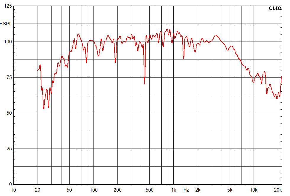
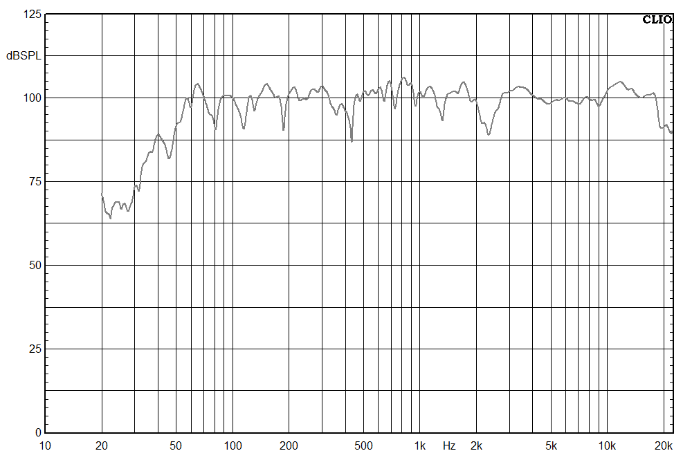
Displayed below is the on-axis measured frequency response of the 8NDL51 without any filters. The response exhibits a natural decline from approximately 4kHz; with a distinct peak at 3.5kHz. This peak aligns itself within the midrange vocal region, which coincides with the area of greatest sensitivity for the human ear. Naturally, we aim to mitigate the prominence of this peak in the final outcome. If the 8NDL51 and Tweeter were to sum constructively at this frequency, the overall sound could be a little harsh. Consequently, our strategy involves selecting a low-pass filter slope that effectively attenuates the 3.5kHz peak.
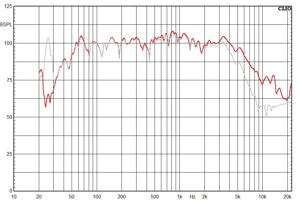
For the purpose of comparison, we started our experiment with a conventional Butterworth 12dB low pass filter at 2500Hz, calculated using default 8 ohm value for impedance. It’s worth noting that the bump down at 30hz was caused by background noise whilst measuring, and should be disregarded. The measured frequency response doesn’t look like the filter is actually working at 2500Hz -this is partly due to the peak at 3.5khz, but also due to the fact that the impedance of the woofer isn’t 8 ohms at the crossover frequency, so the calculated component values wont actually make a Butterworth filter, and will also shift the filter frequency a little higher. This was expected, but we took this step anyway as part of the process to show that default crossover values calculated for 8 ohms will often be incorrect.
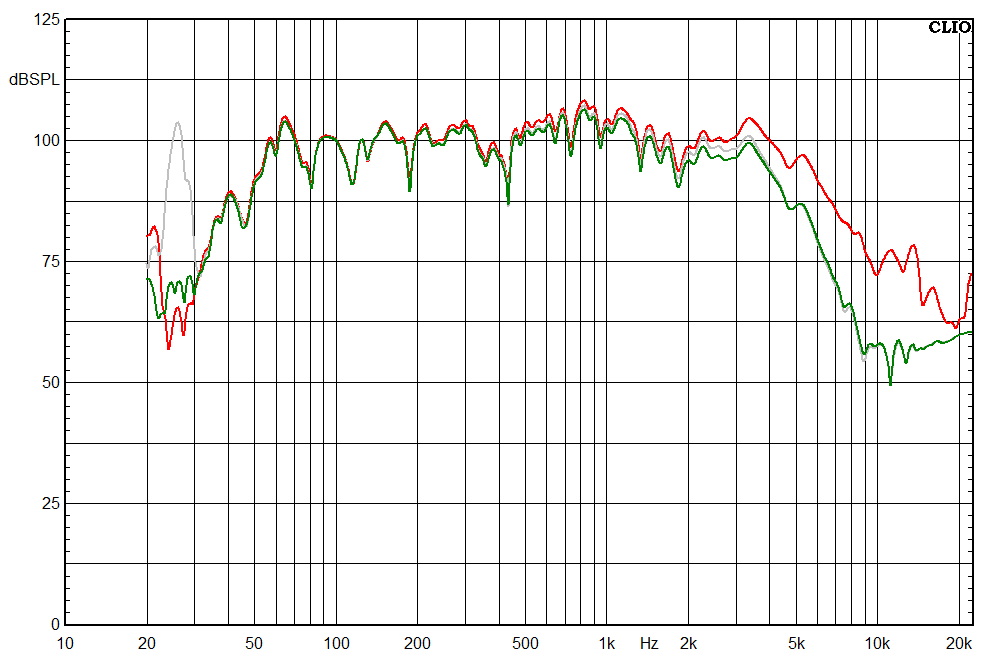
To progress further, we conducted another measurement using a standard Butterworth 12dB filter at 2500Hz. However, this time the calculations were based on an 11 ohm impedance, which is the actual impedance value we’re working with. The outcome of this measurement is illustrated in green in the graph. This adjustment has led to a subtle reduction in the range between 2000Hz and 3000Hz. However, the peak around 3500Hz persists, and the response doesn’t exhibit a substantial decline until after this peak. In order to achieve a satisfactory final outcome, we need to address this peak.
From experience I’m aware that peaks within the range of 1500Hz to 4000Hz could result in a somewhat shrill sound. While it’s acceptable to rectify this issue using a graphic equalizer, I prefer, whenever possible, to devise crossover designs and opt for components that preemptively mitigate these unfavorable peaks.
At this point, it’s pretty common to start playing around with a bit of trial and error to find the right filter that works for getting the woofer’s sound just right. Normally, I kick things off by tinkering with various filter frequencies, gradually going lower until peaks are sufficiently suppressed, and also experimenting with either Butterworth or Linkwitz-Rileyalignemtn . This step-by-step process helps us dial in the woofer’s sound.
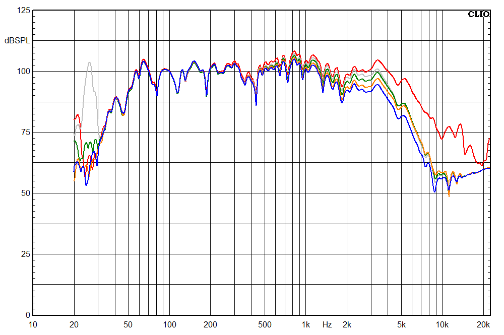
The orange plot is a Linkwitz-Riley 12dB filter at 2500Hz, calculated with 11 ohm impedance, and the blue plot is Linkwitz-Riley 12dB filter at 2000Hz, also calculated for 11 ohm impedance. The peak at 3.5kHz is being gradually suppressed, and getting closer to the frequency response I want from the 8″ woofer.
In the final test, I experimented with a 12dB Butterworth filter set at 1.65kHz, with calculations based on an 11 ohm impedance. The result is represented by the purple plot. It’s getting a bit busy, with multiple results, and I omitted a 4 or 5 other test results which would have made the graph undecipherable. Here’s what’s happening in the final test: this response is a tad louder around 2000Hz compared to the blue plot, but then it takes a steeper plunge after that 3.5kHz peak, which is about as good as I can hope for.
Instead of the typical 2.5kHz low pass filter calculated for 8 ohms, we opted for a 1.65kHz low pass filter calculated for 11 ohms. And already, you can see this is shaping up to be something more bespoke than your standard off-the-shelf crossover. A 2.5kHz low pass would utilise a 0.72mH inductor and 5.6uF Capacitor, we ended up with 1.5mH and 6.3uF – significantly different.
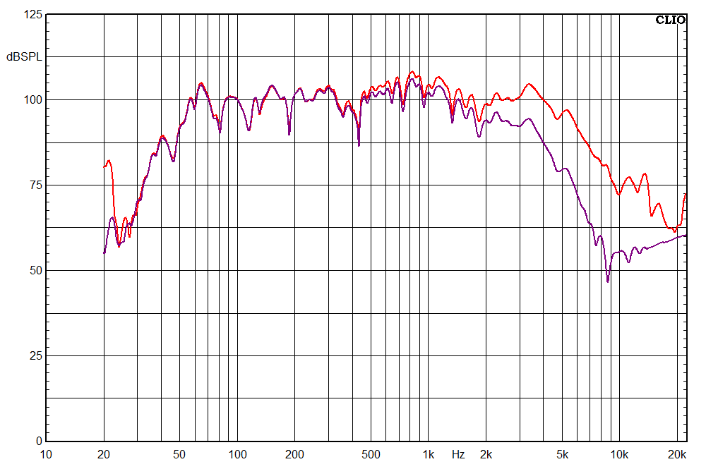
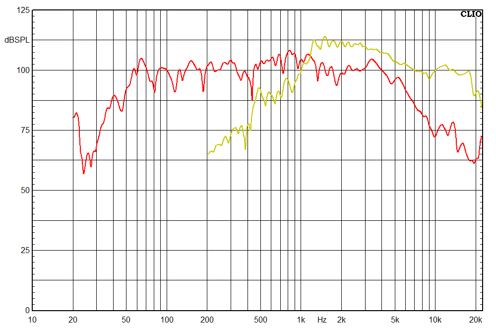
To make things a little easier to see, in the graph below the red plot is the original frequency response of the woofer, and the purple plot is the final low-pass filter we decided to use. We needed the woofer response around 2.5kHz to be lower compared to 1000Hz and under , as the woofer’s response will couple with the tweeters response around this frequency.
Using the lower filter frequency of 1.65kHz has had the added benefit of attenuating the response around 500-1000Hz and bringing it more level to the response between 50hz and 200Hz. This will benefit the final result by allowing for a more balanced mid-range response.
So reaching this decision on the low pass filter for the woofer has been influenced by the impedance measurements of the woofer, which resulted in a different impedance being used for the crossover calculations. In addition to this I have looked at the frequency response and aimed to smooth the mid response and suppress any large peaks on the response. I have used past experience to judge the result from the 8″ I am aiming for, and settled on a solution once the response is looking close to what I am aiming for.
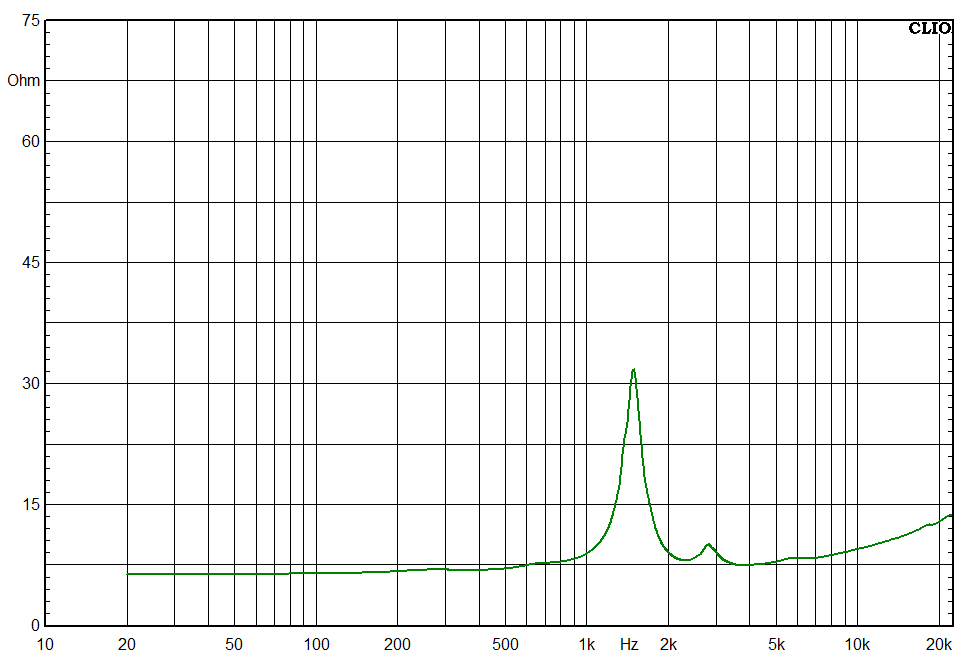
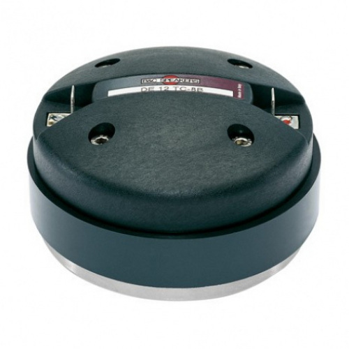
Now we move on to the tweeter. For this project we chose the B&C DE12TC, and repeated the same process of measuring impedance and frequency response. You’ll notice the frequency response plots dont got down to 20Hz, we changed the cut-off frequency as we don’t want to put bass frequencies into a tweeter.
DE12TC Impedance measurement:
Again we have bumps in the impedance of the tweeter, however tweeters are more problematic, as the impedance bumps are often very close to the crossover frequency. The vary impedance cant interact badly with a passive crossover. These impedance bumps are caused by natural resonant properties of the tweeter, and personally I find if the crossover point is too close to one of these bumps the sound is not particularly nice. So I try to keep the crossover points away from the impedance bumps. Again we have the same problem of not being sure what the impedance is at the crossover point, we have a peak of around 10.5 ohms just below 3khz, dropping down to 7.5 ohms and then slowly rising again. This is why impedances are stated as ‘nominal’ – they are just a vague average over the operating frequency range.
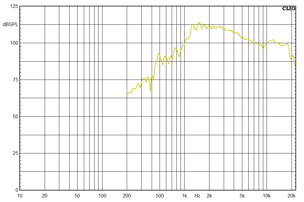
Below is frequency response of the DE12TC.
This might not be the smoothest response, but it’s quite par for the course with most compression drivers. The good news is that nothing here is beyond refinement with a touch of EQ. However, I usually try to work in attenuation and EQ directly into the crossover. This helps harmonize the woofer and tweeter in a way that minimizes the need for extra EQ down the line.
But let’s take a step back. Our first task is to examine the frequency response of both the woofer and the tweeter, and then compare the two. This comparison will give us a solid foundation to figure out the best approach for smoothing out the frequency response of the tweeter so that it blends seamlessly with the woofer.
The first thing that stands out is how the DE12TC is considerably louder than the 8NDL51 from 1kHz to 5kHz – up to 12dB louder (if dB isn’t your thing, just know that 3dB is like doubling the measured sound pressure, and around 10dB is what our ears sense as twice the loudness). If we leave this as is, the end result will likely be a pretty intensely harsh tone with an excessive amount of midrange. To tackle this, we’ll need to dial down the tweeter’s volume to get things balanced.
It’s common, in fact recommended, to utilize an L-Pad arrangement for attenuating high frequencies. This technique is theoretically sound as it facilitates both effective attenuation of high-frequency response and stabilization of the load impedance within the High Pass Filter circuitry. I rarely use L-Pads, and I’ll explain why.
When I build high power crossovers, for speakers of perhaps 600W-1000W, there can be 50-200W of power being directed to the compression driver, sometimes even more in extreme cases. If the compression driver is 9-12dB more sensitive than the woofer (not unusual) you may need to dissipate 100-150W of this power in the resistors. I have cooked enough aluminium clad resistors to have reached the conclusion this is just a bad idea. Dissipating lots of power in resistors invariably leads to reliability issues caused by overheating.
My solution? Use a series resistor. There will be heaps of people that will tell you its a bad idea, but its commonly used in many commercial applications, and power dissipation is the reason. If you need fairly heavy attenuation on an 8 ohm compression driver, you can put another 8 ohm resistor in series with it. The series resistor takes half the power, tweeter takes the other half – but then you have a 16 ohm load. If you know your power calculations, the maths is simple, double the impedance, halve the current. Power = Impedance x current squared. With half the current, you have a quarter of the power, which very effectively reduces total power without having to dissipate loads of heat in resistors.
For serious watts, you can use 2 resistors, spreading the power dissipation over both resistors, and managing the power tidily. There are a couple of drawbacks – first is the fact that the amount of attenuation is proportional to the impedance of the tweeter, so the attenuation will work nicely on this tweeter above 2.5kHz, but not so well below this, as the tweeter has variable impedance (not 8 ohms!) Additionally the combination of impedance bumps, and series resistors messes with the crossover frequencies, particularly the knee in the bend of the high pass filter, as you have variable impedance in the region the filter is transitioning to the pass band, so you end up having to redesign your high pass filter around the attenuation and the new load impedance
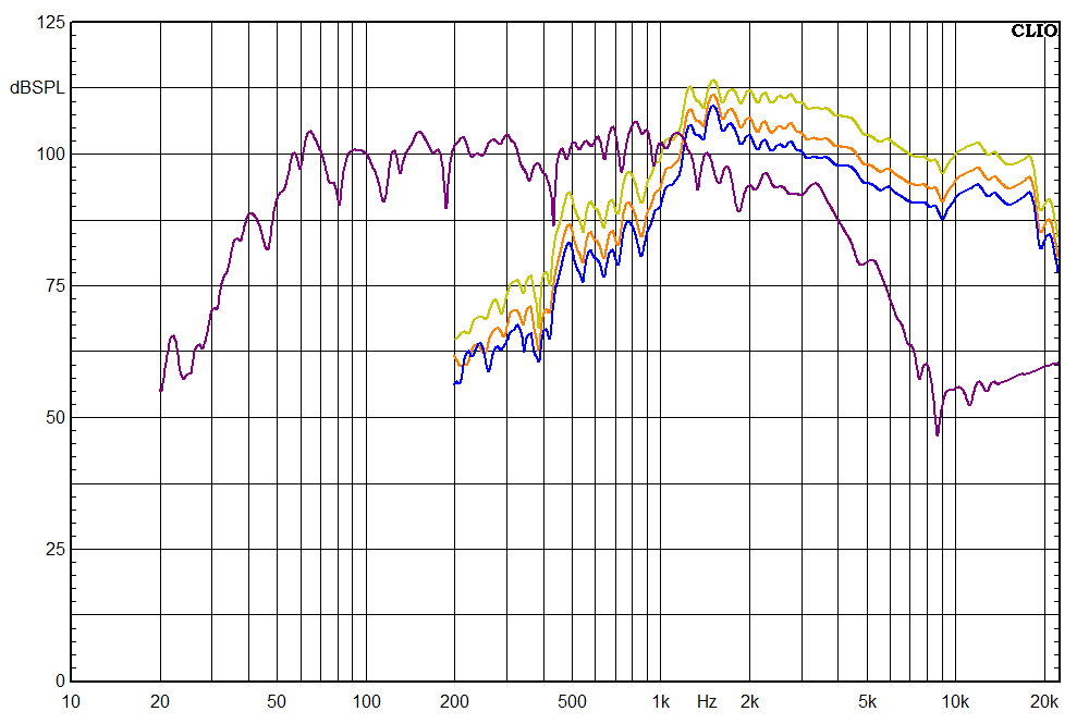
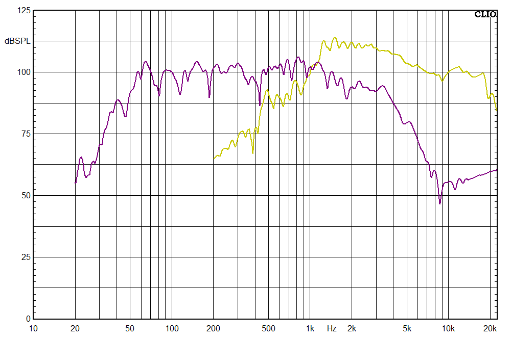
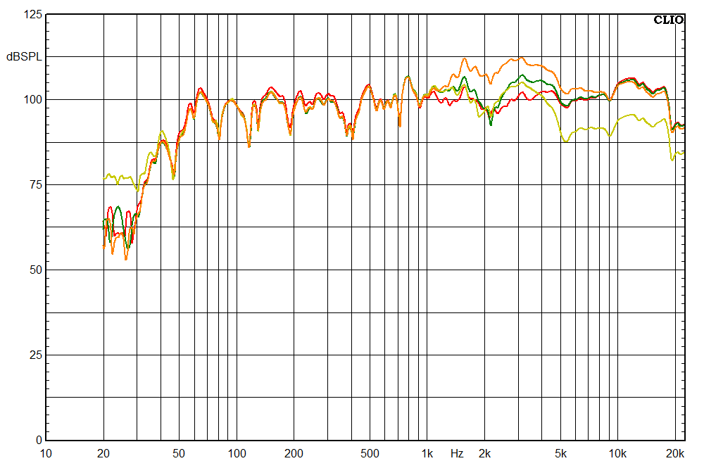
We did some trial and error tests, to work out roughly what attenuation would help balance the sound. The orange plot is with approximately 12 ohms series resistance, and the blue plot is with 24 ohms. There is a noticeable peak at 1.6khz, but we would hope to eliminate this once we have applied a suitable high pass filter. For comparison, the purple plot is the response of the 8″ woofer with the 1.65kHz Butterworth filter applied, and its this purple plot we need to get the tweeter to align to smoothly
Having worked with compression drivers like these before, I skipped a few steps here and just went straight for a filter alignment I expected to work which was a 3.3kHz Butterworth filter This should flatten the response between 1khz and 3khz. You’ll notice also the response is tailing off from around 4khz, due to the fact we are attenuating the high frequencies too much, so we added a 3.3uF bypass capacitor in parallel with the series resistors. This has the effect of adding a hi-shelf EQ to the response, the idea being that you get attenuation below 3-4khz, but at higher frequencies, the attenuation is bypassed by the capacitor, allowing the tweeter to operate at its natural level. If you check out the grey plot, you can see this has worked quite effectively. I could have bored you with multiple iterations of different filters here, so we basically skipped 5-6 tests by utilising past experience.
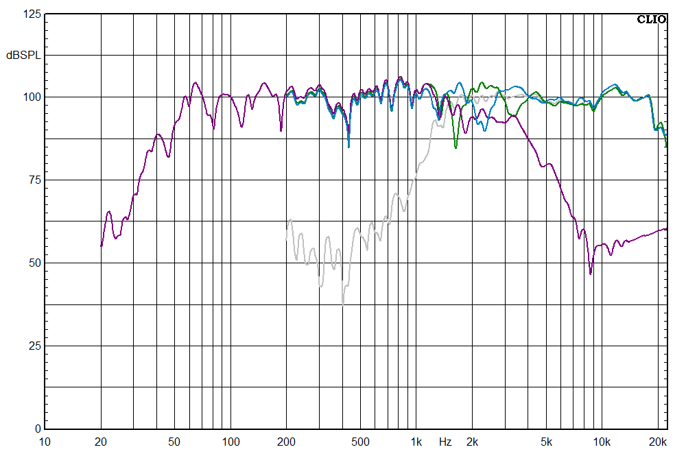
At this point we have added a filter and some EQ, and converted the natural response of the tweeter (yellow-green) to a flatter response (grey). Things are looking quite promising here, but what we have are two independent measurements, purple for woofer, grey for tweeter, but this is not a system measurement of the two together. The next result shows the frequency responses with woofer and tweeter together as a system.
Taking a closer look at the crossover region, there are 2 plots, one green and one blue. Green was with the tweeter in standard polarity, and blue with the tweeter with inverted polarity. Inverting polarity is usually necessary due to phase shift cause by a filter. If we had used a 2.5khz Butterworth high pass and low pass, we would normally run the tweeter in reverse polarity to counteract the phase shift in the crossover. The frequencies chosen: 1.65khz and 3.3khz, are an octave apart, and in the past we have found that having the filter frequencies exactly an octave apart means you don’t need to invert the polarity of the tweeter, and the phase response across the crossover region remains fairly linear. Sadly in this instance it didn’t work. In fact neither configuration worked particularly well. There are other factors, the physical position of the horn makes a difference -you want the voice coils of woofer and tweeter in the same vertical plane to avoid the need for time alignment. Despite trying to ensure the components were arranged correctly, and trying a few subtle variations of crossover components, we couldn’t quite get the flat response we were after. The end result was by no means awful, but there is a noticeable dip at 2.5khz which we just couldn’t rectify using this design approach. The best final frequency response we could achieve is below.
So the response has a few bumps, but we have a working design, which is potentially good enough for some applications. In fact I have had people request that we intentionally put in a slight dip in the frequency response between 1khz and 3khz to give a slight smiley face EQ effect. In this case, the dip is around 10dB, a little more than I would like. I have had very good results with this approach in the past, and got some very smooth sounding speakers, but in this instance it just wasn’t quite right so I decided to go back to the beginning and take a different approach. I went back to the frequency response of the tweeter, to take a closer look, and consider an alternative approach. At 5kHz and above, the tweeter is approximately equal in output to the median level of the woofer. Below 5khz, it gradually rises in output, until its around 12db higher at 2.5khz. This is a pattern I have seen before, and already know how to deal with.
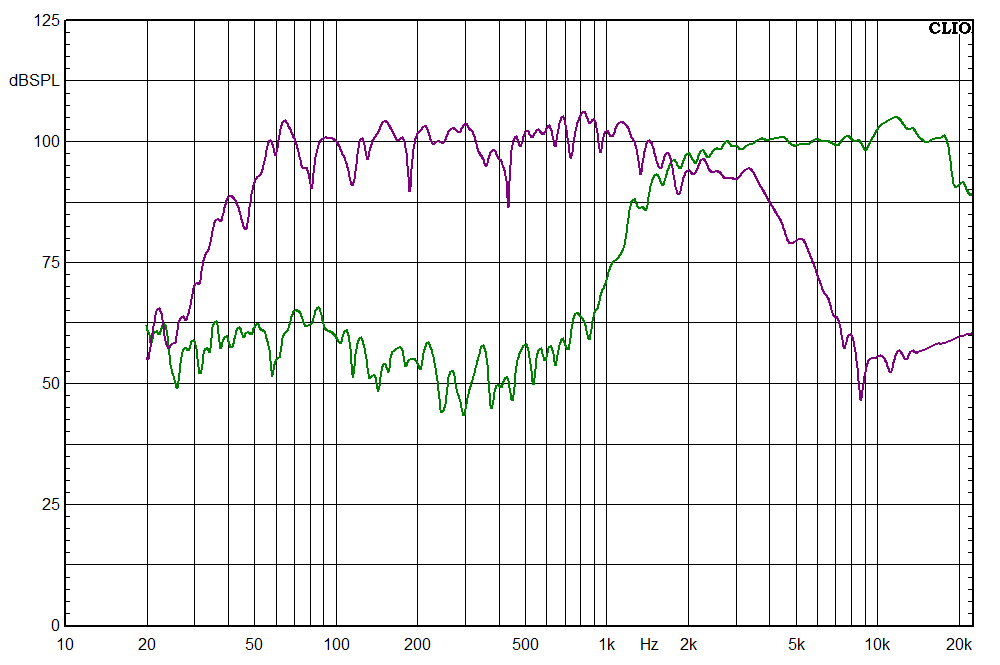
The downward slope of the tweeter’s response is approximately 12db over an octave, exactly the opposite of the slope you would get from a second order high pass filter. Applying a 12db/octave high pass filter at around 5khz, we can effectively rebalance the response of the tweeter, flattening it below 5Khz. Here we have the plots of the 1.65kHz low pass applied to the woofer (purple) and a 5kHz (approx) high pass applied to the tweeter (green). You can clearly see the high pass filter has done its job and flattened out the response from the tweeter.
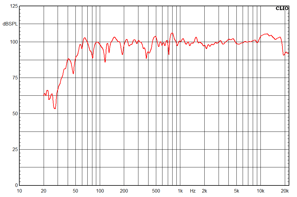
This is looking very promising, shifting the filter point up to around 5kHz has created a fairly flat response from 2.5kHz to 10kHz on the HF device. There is a small peak just above 10kHz, which isn’t a bad thing usually, and will give a little HF sparkle at the top when listening directly on-axis. I did do a few iterations of small filter tweaks and measurements after this, and ensuring the physical positioning of components was just right, but eventually got the result we wanted in the red plot below:
Yes we know its not completely flat. As mentioned at the outset, the environment was such that room anomalies would feature in the measurements. The aim here was to make a crossover that balanced woofer and tweeter, and had a smooth transition from woofer to tweeter without any massive peaks or troughs, which has been achieved.
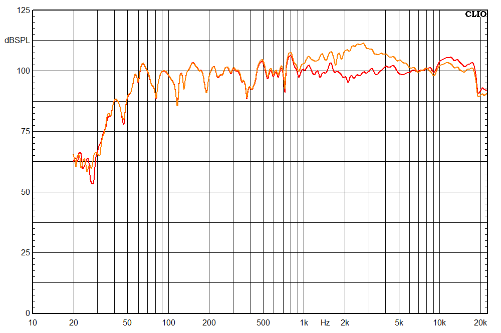
Going back to the reason for writing this article basically to show how standard off the shelf crossovers don’t usually work, we did a measurement with a standard 2.5khz Butterworth crossover calculated for 8 ohm components, you can see the result in the orange plot:
If you understand the graph, you’ll be getting the earplugs ready. It has the potential to sound pretty awful with a 12-15db hill across the midrange and lower hf which will require significant EQ adjustment to rebalance.
The yellow-green plot below is with attenuation resistors added to the tweeter on thedefault 2.5khz crossover, whichjust seems to be introducing more problems. The orange plot is slightly different here, in the previous graph I recalled a measurement with a different mic position. The fact that the frequency response has changed a fair bit from just a small change in mic position is an indicator of phase response problems in the crossover. Basically the woofer and tweeter are not aligned, and in some listening positions will couple constructively, and in other positions couple destructively, causing hot spots within the listening area. The key point here is that the route we are going down, with the off the shelf crossover is not shaping up to be a good solution, despite us trying to make adjustments to rebalance the sound
Whilst I knew I was heading down a dead end, for purposes of completing the test, I added a 3.3uF bypass capacitor on the attenuation resistors, to bring back the upper HF, this is shown in the green plot. Its a little better, but there is a sharp dip at 1.8kHz and a lump at 2.5kHz which are both undesirable, and not as good as the red plot. A lower value capacitor, such as 2.2 uF or 1uF would tame the 2.5kHz bump, but I already knew there were phase response issues with this solution. A little more refinement, and potentially I could have got the 2.5kHz off the shelf default crossover sounding OK on-axis, but I know it would have had issues off-axis.
So its clear that the best frequency response has been obtained using a customised crossover following non-standard practices. At the outset, we were considering a standard 2.5kHz crossover. We ended up with a 1.65kHz low pass and high pass around 5kHz, but with the intent of flattening the frequency responses of the devices. There will probably be critics of this approach, as it doesn’t follow the text book methods everyone has been preaching for years. However, its a simple solution, requiring fewer crossover components, keeping size and cost to a minimum. Also, it works, and works quite well – so why not use it? I have seen similar crossovers used in ‘audiophile’ speakers costing many thousands of pounds. It may be possible to make a better crossover incorporating a zobel network, a large oversized L-Pad attenuator, and possibility using third or fourth order filters -the resulting crossover board could easily end up being larger than the speaker cabinet. This design approach provides for a compact crossover, which can be easily fitted inside a typical 8″ + 1 ” speaker cabinet.
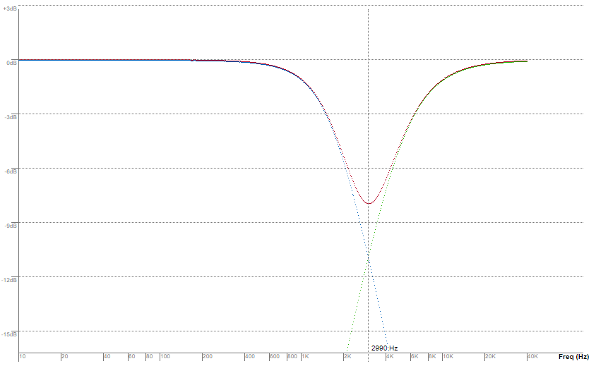
Using a circuit simulation tool I wrote, I put the final design components in and produced the graph below. The tool calculates the attenuation of the filter from the component values and impedance entered, allowing you to calculate the theoretical frequency responses of the filters, and the summed acoustic power response. The result shows the attenuation relative to 0dB of the high pass (green) and low pass (blue) sections. It also shows the summed response in red (ignoring any phase response issues). The ‘crossover’ point works out to be around 3kHz – this is where the high pass and low pass have equal attenuation. Usually the crossover point is defined as the -3dB point of the high pass and low pass filters in a standard crossover. The net result of this circuit design is to put a 7-8dB attenuation across the mid band centered at 3kHz, effectively counteracting the bump in frequency response from the woofer and tweeter when used with a standard off the shelf crossover.
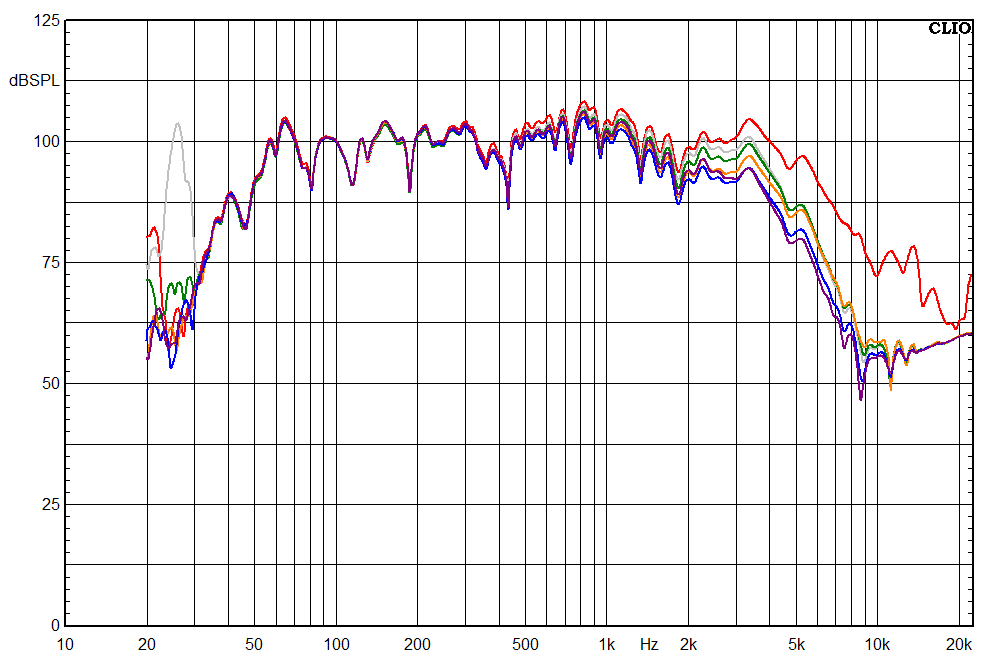
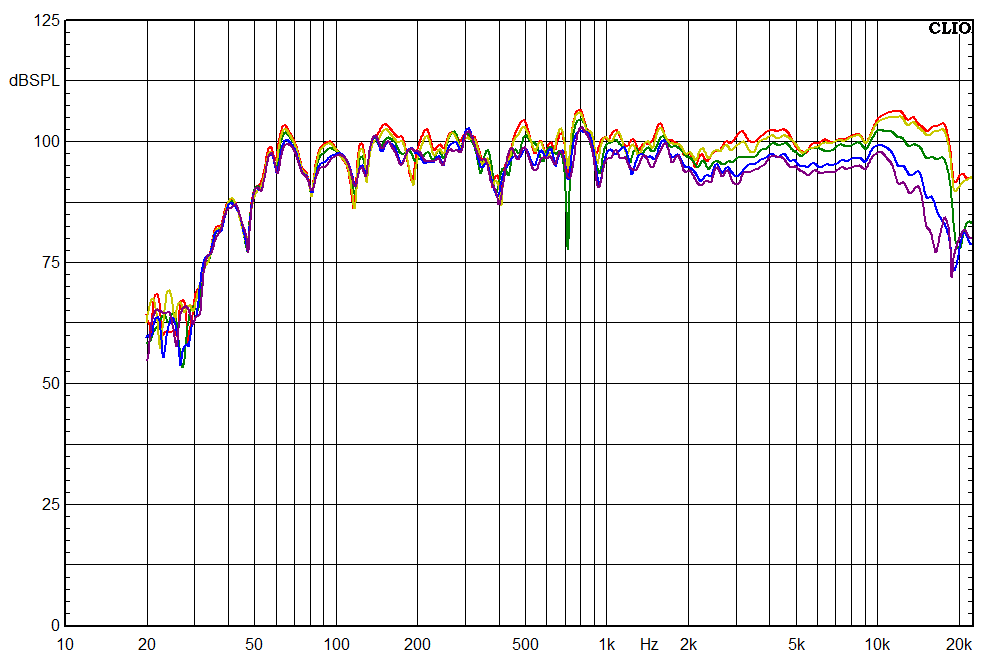
Just to bring things to a conclusion, I thought I would make some extra measurements, to check the speaker performance off-axis. Usually – if there are issues in the phase response of the crossover, which prevent the woofer and tweeter working in harmony, when you move the measurement mic off axis and repeat measurements, you will encounter peaks and troughs at various frequencies. Below are the various responses measured: Red is on axis, Yellow is approx 10 degrees off axis, Green approx 20 degrees, Blue around 30 degrees and purple around 45 degrees. The plots follow the expected results, where the wave guide on the HF device is controlling the dispersion, and the higher frequencies gradually get quieter off axis. The slightly higher response of the HF above 10khz is tamed when listening off axis to help maintain a good sound from multiple angles. Overall I am pleased with the result. All that’s left is to build a prototype cabinet and get some listening tests done.
The process of measuring, trial and error testing, simulations, and repeated iterations can take anything from 15 mins to several hours for each crossover. It depends on how well the woofer and tweeter interact with each other, and whether different approaches offer suitable solutions. Sometimes things just don’t work, and wont work, and no amount of iterations gets a good result – this usually means the wrong drivers have been selected that just don’t want to work together. Initially I started doing crossover designs this for personal research only, but I do offer custom crossover design as a service, with limited availability. It can be a fairly involved process, so the time and effort required needs to be justified, and its simply not viable to do it for everyone who asks. Additionally, I can only do this for components I have access to. If I don’t have the components, I cant measure them, and I can’t test the possible solutions. For best results, I also need the finished cabinet; the position of the drivers with respect to each other, the front baffle design, and other factors all affect the frequency response. Even a grill attached to the front can have an noticeable effect on the HF response, so to get this ‘exactly’ right – its best to have everything exactly as it would be in a finished cabinet. Its is absolutely impossible to design a custom crossover theoretically, you have to be able to measure and test in order to refine the solution.
For anyone who fancies building themselves a super high quality speaker, the components for this project are:
B&C 8NDL51 (8 ohm)
B&C DE12TC (8 ohm)
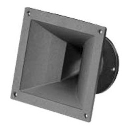
B&C ME15 horn flare
and a custom crossover:
L1 = 1.5mH
C1 = 6.3uF (5.6uF + 0.68uF)
L2 = 0.51mH
C2 = 1.8uF
This design isn’t intended for massive bass response, but you can get sensible levels of bass down to around 50-60Hz at medium volume with the cabinet tuned right. For best results at higher volumes you would need a separate subwoofer.
Qts is one of the most critical Thiele-Small parameters when designing a speaker system. It represents the total quality factor of a driver, combining both electrical damping (Qes) and mechanical damping (Qms) into a single value. Understanding Qts is useful for determining the best type of enclosure for a driver. Getting the right Qts for a bass reflex enclosure ensures efficient output, strong transient response, and extended bass performance.
What Exactly Is Qts?
Qts is a dimensionless number that describes how well a driver controls its own resonance. It is calculated using the following formula:
Where:
Qms = Mechanical quality factor (how well the suspension controls cone movement)
Qes = Electrical quality factor (how well the voice coil and magnet control movement)
A lower Qts means more damping, resulting in tighter, more controlled motion. A higher Qts means less damping, allowing the driver to resonate more freely. A higher Qts driver tends to demand a larger cabinet to operate most effectively, so choosing the right driver with the right Qts is very important for almost every speaker cabinet design.
The Best Qts Range for PA Speakers
For PA speakers, especially bass reflex (ported) enclosures, the ideal Qts range is:
✅ 0.30 – 0.45 → Best for ported PA subwoofers & woofers ✅ 0.35 – 0.38 → The sweet spot, balancing efficiency, transient response, and bass output ✅ Above 0.45 → Can still work in ported enclosures, but requires a larger cabinet
A Qts below 0.3 is generally found in horn-loaded enclosures, where tight cone control and efficiency are prioritized, and the driver will work happily with a small rear chamber. There are sometimes exceptions, these are intended as guidelines only, to help make an informed choice if you’re just starting blindly at a wall of numbers.
How Qts Affects Ported Enclosures
Qts 0.30 – 0.38 → Balanced sound with good transient response and deep bass.
Qts 0.38 – 0.45 → More extended bass possible, but less transient snap.
Qts above 0.45 → Requires a larger cabinet to compensate for weaker motor control.
For PA subwoofers and woofers, the ideal Qts keeps the cabinet size reasonable while ensuring powerful, clean bass.
PA Speaker Examples
Driver Type
Typical Qts Range
Best Enclosure Type
PA Subwoofer (Ported)
0.30 – 0.38
Bass Reflex (Ported)
General PA Woofer
0.35 – 0.45
Ported, some larger designs
Horn-Loaded Subwoofer
0.15 – 0.30
Horn-Loaded
🔹 Example 1: A Qts = 0.35 subwoofer is ideal for high-efficiency ported enclosures, delivering tight, punchy bass. 🔹 Example 2: A Qts = 0.42 woofer can still work in a ported cabinet, but may require a larger box to compensate. 🔹 Example 3: A Qts = 0.20 subwoofer would likely underperform in a ported box, but excels in a horn-loaded design.
Final Thoughts
For PA systems, getting the right Qts for a ported enclosure is crucial.
✅ The sweet spot for PA ported enclosures → 0.35 – 0.38 (from our experience) ✅ Avoid Qts above 0.45 unless using a very large cabinet ✅ Below 0.3 is best suited for horn-loaded designs
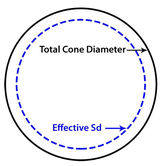
Sd (Effective Diaphragm Area) is the active surface area of a speaker cone that moves air to produce sound. It’s usually measured in square meters (m²), but sometimes also specified in square centimeters (cm²). Sd is most often used for calculating other TS parameters, and its fairly common for all woofers with a certain diameter to have virtually the same Sd, this is because it can be calculated directly from the speakers diameter:
Where:
Sd = Effective diaphragm area (m²)
D = Effective cone diameter (meters)
π (pi) = 3.1416
Note: The effective diameter usually excludes the surround—only the part of the cone that actively moves air is considered – this can be hard to determine in some cases as some of the surround does move with the cone. For precise Sd, advanced methods are required to accurately determine the active surface area.
Rms, or mechanical resistance, describes how much damping the speaker’s suspension provides to control cone movement. Think of it like shock absorbers in a car—too much resistance, and the suspension is stiff and unyielding; too little, and it becomes too loose, leading to uncontrolled movement.
Rms is directly linked to Cms and Fs, as can be seen in the formula below:
What Does Rms Actually Do?
Rms affects how quickly the cone stops moving after being displaced. A higher Rms means more damping, which helps prevent unwanted resonances but can reduce efficiency. A lower Rms means less damping, allowing for more movement but potentially leading to excessive ringing or overshoot.
How Rms Affects Speaker Performance
Higher Rms (More Damping) →
The cone stops moving quickly after a signal ends
Prevents excessive ringing and improves transient response
Often found in PA and midrange drivers, where control is crucial
Can reduce efficiency because more energy is absorbed
Lower Rms (Less Damping) →
The cone moves more freely, leading to longer decay times
More efficient at converting electrical energy into sound
Often found in subwoofers, where extended low-frequency response is desirable
May require careful tuning to avoid unwanted resonances
How Rms Relates to Qms
Rms directly affects Qms, the mechanical quality factor of a driver.
A low Rms results in a high Qms, meaning the driver has lower mechanical losses and rings for longer.
A high Rms leads to a low Qms, meaning mechanical energy is dissipated more quickly, reducing ringing.
For example:
A PA midrange driver may have Rms = 5 kg/s and Qms = 2-3 for precise, controlled response.
A subwoofer may have Rms = 1.5 kg/s and Qms = 7-10 to allow for more free movement and extended bass.
Rms and Speaker Efficiency
Higher Rms means more energy is absorbed as heat in the suspension, making the driver less efficient. That’s why high-efficiency speakers (like horn-loaded designs) often have low Rms, reducing mechanical losses.
Real-World Example of Rms in Different Drivers
Driver Type
Typical Rms (kg/s)
Effect on Performance
PA Midrange
4 – 6
Tight control, minimal ringing
Hi-Fi Woofer
2 – 4
Balanced damping for clarity and bass extension
Subwoofer
1 – 2
More excursion, deeper bass, less damping
Final Thoughts
Rms might not be the most commonly discussed Thiele-Small parameter, as typically most people focus on Cms or Vas. These are ways of quantifiying more or less the same thing, just in slightly different ways.