Science of Sound Archive

POWER – What’s a watt?

Posted By Andy Kos

Over the years in the audio industry, I have made numerous attempts to explain some of the concepts used with regard to speaker/amplifier power. Most are summarised below, with links to some of the articles covering each topic in more detail. If you’re serious about sound, and curious about power, these are well worth a read, and will help you make more sense of power.

What is Power (Watts)?

Power is a measure of how fast energy is being used or delivered. One watt is defined as one joule per second, which in audio terms is the rate at which energy is transferred from an amplifier to a loudspeaker. High power for a short burst and lower power delivered continuously can result in the same total energy, which is why power must be considered over time.

For example, a 4 W burst for 0.25 seconds followed by 0.75 seconds of silence delivers the same energy as a 2 W burst for 0.5 seconds followed by 0.5 seconds of silence, or 1 W delivered continuously for 1 second.

This simplified example is an analogy for understanding peak, program, and continuous power. Peak power represents short, high-energy bursts, program power represents longer bursts with more time at a high level, and continuous power represents energy delivered without breaks. Although real music does not follow fixed duty cycles, all three cases above average to the same energy rate: 4 W × 0.25 = 1, 2 W × 0.5 = 1, and 1 W × 1 = 1.

This is why loudspeaker power ratings typically follow the same pattern: program power is usually twice the continuous rating, and peak power is typically four times the continuous rating. The numbers relate to the same underlying energy, but describe how that power is delivered over time.

RMS Power

RMS is a mathematical method that works extremely well for steady sine waves, such as AC mains power, where voltage and current are continuous and predictable. Music is not like this, so “RMS power” is not ideal for describing real audio behaviour. Some amplifier manufacturers still use the term, but it often includes a hidden crest factor or burst condition, meaning the figure is not a true continuous power level but a calculated equivalent.
Read more…

AES / Continuous Power

AES power defines how much power a loudspeaker can handle on average over time using a standardised broadband noise signal. It represents the long-term thermal limit of the voice coil and is the most reliable figure for continuous operation. Unlike RMS-style ratings, AES power is designed specifically for real audio signals rather than steady test tones.

Program (Music) Power

Program power allows for higher short-term peaks while keeping the long-term average power the same as the AES rating. It reflects the dynamic nature of music, where loud transients are followed by quieter moments. Program power is headroom, not extra continuous power, and should never be treated as a sustained operating level.
Read More on AES / Program Power

How much Power do you need?

What’s up with the Watts?
Power ratings in audio can be confusing because music is dynamic, not constant. Its hard to know what you want, what’s best and how to use power figures sensibly when choosing speakers and amplifiers.
Read More…

Pe – Power Handling Capacity

Often seen in manufacturers technical data, Pe is the long term power handling capacity, usually measured using the AES standard (but not always) and some manufacturers have their own test criteria and will often name this ‘nominal power handling’ This is not necessarily comparable between all speaker brands – also a little explanation as to why MORE POWER does not necessarily mean MORE VOLUME
Read More..

RMS Power

Posted By Andy Kos

What does RMS actually mean?

RMS stands for Root Mean Square. It is a mathematical method, not a type of power. It is normally applied to voltage or current, but for many years it has been used in the audio industry to describe amplifier and loudspeaker power.

Why? Simply because it was the best available method at the time, and no better, widely agreed standard existed.

I am often asked “What’s the RMS power?” My usual answer is that RMS is not particularly suitable for audio. If you want to understand why, read on. Otherwise, just accept that AES power is the standard you should be using for loudspeakers.

Why do we have RMS at all?

RMS comes from electrical engineering, where it works extremely well for AC power systems. It allows an AC signal to be converted into an equivalent DC value that produces the same heating effect.

In the UK, mains electricity is described as 240 V AC. That figure is already an RMS value. In reality, the waveform swings to about 339 V peak, or 679 V peak-to-peak.

The RMS figure is very useful. If an electric heater draws 10 A from a 240 V supply, we call it a 2400 W heater. The voltage and current are constant, the waveform is a steady 50 Hz sine wave, and the power delivery is continuous. This is a perfect use case for RMS.

[Image: AC sine wave showing peak, peak-to-peak, and RMS level]

Why RMS doesn’t map cleanly to audio

Audio amplifiers and loudspeakers do not operate with constant sine waves. Music is dynamic, the amplitude changes constantly, and power delivery is anything but steady.

To work around this, various test standards were created using controlled noise signals instead of tones. For loudspeakers, common examples included EIA RS-426A and IEC 268-5.

With a known test signal, it is possible to calculate an equivalent RMS value using averaging and squaring maths. This is where the idea of “RMS power” for speakers came from. However, it was never especially accurate, and often resulted in unrealistically low power ratings.

The amplifier vs speaker mismatch

Over time, it became normal to match amplifier and speaker ratings directly. For example, using a 400 W RMS amplifier with a 400 W RMS speaker.

The problem is that the two numbers were not measuring the same thing.

Amplifiers were often tested at 1 kHz using a continuous sine wave into a resistive load. This frequently overstated real-world power, because at lower frequencies (around 40–100 Hz) the power supply could not always sustain the same output. In practice, usable power at 100 Hz could be 10% lower than at 1 kHz.

Meanwhile, loudspeakers could often tolerate short-term peaks above their RMS rating. This is why users traditionally chose a slightly larger amplifier, to provide headroom.

Conclusion

RMS was not useless, but it was never a complete or accurate way to relate amplifier power to loudspeaker power. There was always an element of estimation and experience involved.

This mismatch is exactly why modern standards moved on, and why RMS power is no longer the best reference point for real-world audio systems.

Making sense of power

Posted By Andy Kos

AES Power, Program Power, and Amplifier Power Explained

Power ratings in audio are confusing because they try to describe something that is constantly changing. Music is not a steady signal, yet power ratings are often presented as if everything operates at a fixed level. To make sense of AES power, program power, and amplifier power ratings, it helps to think in terms of power over time, rather than a single number.

Summary

AES power describes how much power a loudspeaker can handle on average over time. Program (music) power allows for higher short-term peaks, not higher continuous power. Real music delivers power in bursts rather than as a constant load. Modern amplifiers, especially Class D designs, are very good at producing high peak power briefly, while long-term power is limited by heat, power supplies, and mains capacity. The aim of this article is to show how average power, burst power, and time are related, and why a headline figure such as a 2000 W peak can be entirely real while still not representing the long-term power demand of a system. By looking at how music behaves over time, and using simple visual examples, it becomes much easier to understand how loudspeaker ratings, amplifier ratings, and even 13 A mains plugs all make sense in practice.

AES Power vs Program (Music) Power

Modern loudspeaker drivers are usually specified with two related power figures: continuous power (often defined using the AES standard) and program or music power.

AES power represents the long-term average thermal capability of the loudspeaker. It indicates how much power the voice coil can safely dissipate as heat over time using a defined broadband test signal. In simple terms, AES power is a safe long-term operating limit.

Program (music) power is typically quoted as twice the AES power, which corresponds to a +3 dB increase. Importantly, this does not mean the loudspeaker can handle twice the average power. The long-term average power remains the same as the AES rating.

The difference between AES and program power is not extra heat capacity, but crest factor. Program power allows for higher short-term peaks while keeping the long-term average unchanged. The signal is allowed to get taller for brief moments, but not heavier overall.

To understand why this distinction matters, it helps to look at how power is delivered over time.

Power over time: short, high peaks

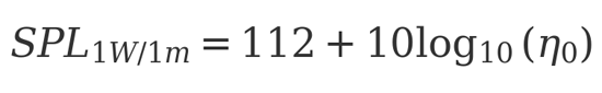
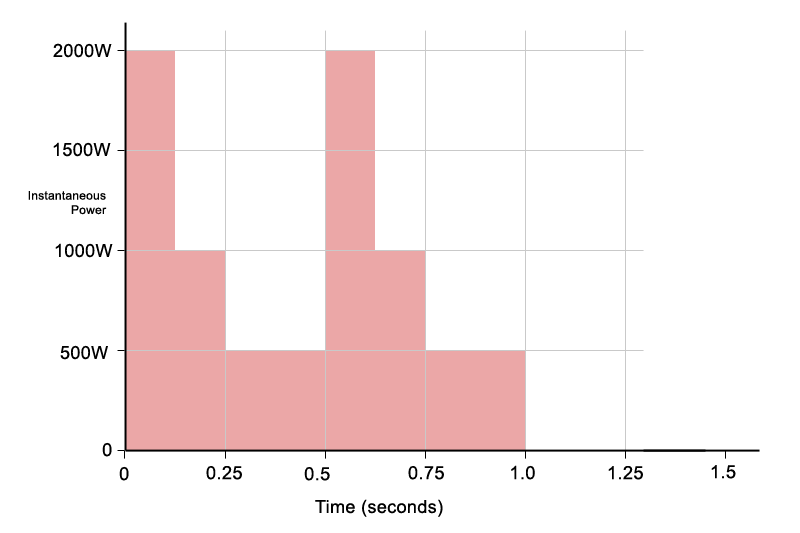
In the first diagram, the vertical axis represents instantaneous power, and the horizontal axis represents time. The shaded red areas show when power is being delivered.

The diagrams are illustrative rather than literal. Their purpose is to explain concepts, not to define exact test conditions or limits.

Figure 1: Short-duration, high-peak power delivered in brief bursts over time.

Each rectangle represents a short burst of power:

  • Peak power: 2000 W
  • Duration: 0.5 seconds

Power multiplied by time gives energy. A 2000 W burst lasting 0.5 seconds delivers the same energy as 1000 W delivered for a full second:

2000 W × 0.5 s = 1000 W × 1 s

Although the instantaneous power is high, it is only present briefly. When averaged over a longer time window, the effective power is much lower. This is the key idea behind program power: higher peaks are allowed, but they do not increase the long-term average.

This type of power delivery closely resembles real music. Bass hits, kick drums, and transients are short, intense bursts separated by quieter moments.

To make the diagrams easier to understand, I have intentionally used simple numbers, 2000W, 1000W, 0.5 seconds – it makes the maths much easier. You can see each red rectangle is divided up into 8 smaller rectangles, which is easy to visualise.

Same energy, delivered differently

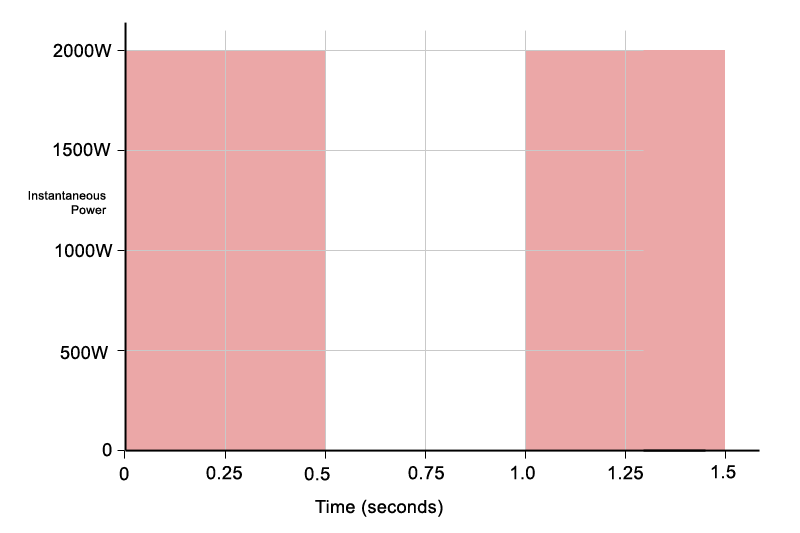
In the Figure 2, the same total energy is delivered in a different way. Instead of short peaks, power is delivered continuously. This is similar to electrical systems such as heaters, power is delivered continuously to a static load, the power level does not go up or down, it remains constant. Music is not like this, amplifier and music power is dynamic, and constantly changing. The power an amplifier delivers to the speaker, and draws from the mains supply varies with time.

Figure 2: The same total energy delivered as lower, continuous power over the same time period.

  • Power level: 1000 W
  • Duration: 1 second

The shaded area is the same size as in the Figure 1, which means the total energy is identical. The average power is also the same. You can see this visually: the area still covers exactly eight grid squares, just arranged differently.

In this example, the continuous 1000 W case does not represent a significant challenge for the amplifier. An amplifier capable of delivering 2000 W peaks will typically have no difficulty sustaining 1000 W continuously, as the average power and thermal load remain well within its design limits.

The real limitation appears when high power is sustained for longer periods. While short bursts of 2000 W are easily achievable, maintaining that level for several seconds places extreme demands on the power supply and output stage. Voltage rails sag, current limiting engages, and thermal protection may begin to operate.

This is where many Class D amplifiers reach their limits. They are designed to deliver very high short-term power with ease, but they are not intended to sustain maximum output continuously, particularly at low frequencies.

What this means for loudspeakers

From the loudspeaker’s point of view, heating depends on average power over time, not peak power. The voice coil does not care whether energy arrives in short bursts or steadily; what matters is how much heat builds up overall.

AES power therefore describes a realistic long-term thermal limit. It represents the average power a loudspeaker can dissipate safely over time without overheating. In the simplified examples shown here, this is illustrated by the second diagram, where the average power level remains constant.

Program or music power acknowledges that real music is dynamic and contains peaks and lulls. This is illustrated in the Figure 3, where the total shaded area remains the same, but the instantaneous power rises to higher peaks. The average power is unchanged, the program material just has a higher crest factor with more pronounced peaks and lulls.

Figure 3: Illustrating crest factor for music/program power.

This simplified example shows how a loudspeaker can safely handle higher short-term peaks, provided the long-term average power remains within the AES rating. Program power just shows the speaker can handle higher short term peaks, as long as the long-term average power remains within the AES limit.

Problems arise when program power is treated as a continuous operating level. If the programme material has little dynamic range, or if heavy compression and limiting are applied, the crest factor is reduced and the average power rises toward the peak level. In this situation the loudspeaker is no longer operating within its intended thermal limits and the voice coil can overheat.

Program power is therefore best understood as a headroom allowance for dynamic signals, not as a sustained power rating. It best represents live music, particularly percussive sounds. Electronic, synthesised music is often compressed, and has long extended bass notes with low dynamics.

What this means for amplifiers

Modern amplifiers, particularly Class D designs, behave much like the first diagram rather than the second.

They are extremely good at delivering short bursts of high power thanks to high-voltage rails and efficient output stages. This is why many modern amplifiers are rated using standards such as EIAJ, which better reflect burst capability and musical crest factor.

What these amplifiers cannot do is sustain very high power indefinitely, especially at low frequencies. Long, continuous bass notes place heavy demands on the power supply, causing voltage sag, current limiting, or thermal protection to intervene.

This is why amplifier power ratings often look impressive on paper but drop significantly under continuous sine-wave testing, particularly into low impedances.

Matching amplifier power to speaker power

Program power is useful when choosing an amplifier because it indicates how much headroom is available for musical peaks. A common and sensible approach is to choose an amplifier capable of delivering somewhere between the AES power and the program power of the loudspeaker.

This provides enough headroom for dynamics without pushing the driver beyond its long-term thermal limits. However, once amplifier power approaches program ratings, proper use of limiters and compressors becomes essential to prevent excessive average power.

How can this make sense on a 13A plug?

The same power-over-time logic also explains why large amplifiers can operate from ordinary mains supplies. To take this one step further, it is useful to look at a more realistic musical signal rather than a simple rectangle, which represents power being fully on or fully off.

Figure 4 shows a simplified ADSR-style envelope, loosely resembling a typical percussive sound such as a drum hit. The instantaneous power still rises briefly to around 2000 W, but the time spent at high power is much shorter than in the rectangular examples.

Figure 4: A simplified percussive envelope showing brief high-power peak typical of a real musical signal.

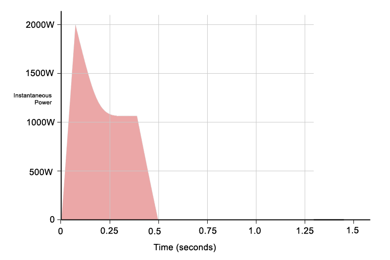
As a result, the total shaded area is smaller, meaning less total energy is delivered overall. Despite the high peak, the average power remains relatively low. This is exactly the type of signal that modern Class D amplifiers handle extremely well: short, high-power bursts delivered cleanly without clipping and distortion. To clarify, this is not intended to suggest that a Class D amplifier cannot sustain peaks for longer than shown – indeed most can. The diagram is simply a representative example of real-world music, intended to show how musical signals translate into long-term average power, and why the ability to handle short bursts of high power is important for preserving dynamics.

This behaviour explains why large amplifiers can produce impressive peak power figures while still operating safely from standard mains connections. The peaks are brief, the average power is modest, and the electrical system only needs to support the long-term average rather than the instantaneous maximum.

For reference, the percussive example above has been approximated into a final diagram (Fig. 5) showing the same energy spread out as continuous power over time. Although the instantaneous peak reaches around 2000 W very briefly, the equivalent long-term average power is much lower, in the region of 600W.

Figure 5: The same energy from Figure 4 redistributed as continuous power, showing the equivalent long-term average.

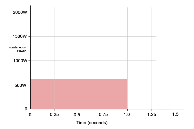
This illustrates an important point: a short, high-power percussive event may look extreme when viewed instantaneously, but when averaged over time it represents a far more modest power demand. Even when additional sounds are present, the medium-term average power may only rise to around 800-900 W.

Applied across a four-channel amplifier, this suggests that even when all channels are working hard, the combined long-term average power is often closer to 3000W rather than the headline peak figures. While this approaches the practical limits of a 13 A mains supply, real music contains loud passages, quieter sections, and natural breaks. These variations reduce the long-term average further, keeping operation within safe limits.

This is why high-power amplifiers can operate from standard mains connections. Peak power figures describe short-term capability, not continuous demand. In the case of amplifiers such as the JAM Systems Q10, which is rated at up to 2500 W EIAJ per channel into 2 ohms, the apparent mismatch between output power and a 13 A plug disappears once power is considered over time rather than at its instantaneous maximum. Realistically this amp is at the limits of a 13A supply, which is why it comes with a heavy duty mains cable with 2.5mm cable and a heavy duty plug.

After being asked countless times how the JAM Systems Q10 can operate from a 13A plug, this article was written to explain exactly that. This article now serves as the standard explanation.

The key takeaway

Power ratings make far more sense when you consider how power is delivered over time. Peak power, program power, and amplifier ratings all describe different aspects of the same thing: short-term capability versus long-term limits.

Many people dismiss peak power figures because of how terms such as PMPO were misused in consumer hi-fi, often wildly overstating real capability. However, genuine high burst power serves a real purpose. It allows the dynamics of the original programme material to be preserved, delivering very large transients when required, but only for short periods of time.

AES power defines what is safe on average. Program power defines how much headroom is available for musical peaks. Understanding the difference makes amplifier choice, system setup, and real-world behaviour far easier to predict.

The Human Ear

Posted By Andy Kos

Something often overlooked, but I believe to be an important part of designing, building and configuring loudspeakers systems is understanding some of the basics of the human ear, and the effects of sound on the human body. This article is intended as a brief introduction, and is by no means exhaustive.

The smiley face equaliser

img1

I’m sure you’ve seen this used, and possibly even done it yourself at some point in time.

Some would argue this is wrong, others that it is right.

The ‘smiley’ face curve often seen on graphic equalisers is similar to the effect achieved by the ‘loudness’ button on many hi-fi systems. It boosts the bass and treble to make it sound ‘better’ – but why do we think it sounds better?

Is it the speakers arent working properly? Maybe… we’ll discuss this later

But is something else wrong?

You might assume your ear works like a high quality studio microphone, with a flat frequency response across the audio spectrum, research has shown this is not the case. The way the ear responds to different frequencies varies considerably.

human ear


The graph above shows lines of perceived equal volume. First thing you will notice is that the smiley face equaliser curve is remarkably similar to the frequency response of the ear, but offset a little with the centre point around 3kHz and more emphasis on low frequencies. To some extent the smiley face can be explained as just naturally compensating for the human ear, making lower volume program material sound like we would expect it to sound at high volume.

Key Points:

Essentially deaf to bass frequencies:  This goes some way to explaining the loudness functions on hi-fi systems, at low volume, we find bass very difficult to hear, and it needs boosting significantly. As the volume increases the curve flattens, requiring less bass boost. In effect the loudness function is giving our ears the same balance as ‘loud’ music, but at low volume. Many people are unable to hear detail in bass frequencies, and some actually prefer the sound of distortion in bass frequencies, as they feel the sound is ‘warmer’

Most sensitive to mid-range frequencies peaking at around 3-4 kHz: Approximately the same frequency as a human high pitched scream or yell, which is not dissimilar to a baby’s cry. This means our ears are most efficient at detecting important sounds, research suggests this is down to years of evolution. Many alarm designers utilise these frequencies to maximise effectiveness. With out ears being so sensitive in the mid frequencies, poor quality sound, particularly distortion will be extremely noticeable, perhaps this goes some way to explaining the smiley curve; a way of masking problems in the mid-band by overpowering with bass and treble? Many people find distortion in the upper-mid frequencies painful, and this is often linked with occurrences of tinnitus.

Response varies with volume: As the volume increases, our ears hear differently. This is one of the reason many high-end large scale PA Systems utilise Dynamic EQ, where the equalisers are programmed to change as the volume increases. If you do apply equalisation to your sound system, you may need to adjust it for low/high volume.

So is the smiley curve correct? In my opinion, most of the time it isnt, particularly if you are playing back pre-recorded music the original recording will have been tweaked by the engineer to sound ‘right’. What is definitely correct is to equalise your system to make it sound right at the volume it is being used, and the room it is being used in, and the type of program material being played through it. If this happens to be a smiley curve, so be it, but as a system operator you should resist the urge to just boost bass and treble in the hope it will sound better. If you find you are doing this a lot, you might want to consider upgrading your sound system.


Be the first to comment

Totally Addicted to Bass?!?

Posted By Andy Kos

Its well known that a heavy bass line is in dance music is often very popular, and many people believe it is absolutely essential in order to create the best atmosphere for certain styles of music, but could we actually be addicted? Some people think it may be possible, and there is some research to suggest they are right.

To understand how this may be possible, we need to understand how sound affects our bodies. In modern life, one of our primary needs to hear is to communicate, often at moderate volume, but our ears can be much more useful than this, allowing us to be aware of things further away than we can see, and some of these things may help explain how our bodies react to sound.

Thousands of years before we had amplified music, bass frequencies, and how we reacted them, could have been critical to our survival. In nature, loud sounds, with an emphasis to low frequencies are often connected to danger. Just think of the sounds created by a stampeding herd of animals, an earthquake or a volcano erupting. Research suggests that years of evolution have developed the ‘fight or flight’ response in humans when presented with danger, this stimulates the production of adrenaline, enhancing the bodies ability to react to the danger.

You’ve heard of adrenaline junkies right? Well, it is possible that the brain associates high levels of bass with pleasure due to the mild adrenaline rush that bass frequencies may cause, and over time, coupled with other stimulants, could contribute to an addiction.

Another field of research suggests exposure to very high sound pressure levels (commonly found in bass frequencies) damages our ears and causes ‘pain’, however our bodies naturally react to this pain by creating numerous chemicals within the body, including adrenaline, endorphines and encephalons, collectively acting to blunt pain, but at the same time causing a pleasure enhancing morphine-like effect. This has yet to be proven, but the theories seem to hold true, and could also contribute to this concept.

One researcher has even gone as far as to suggest that extreme bass frequencies that penetrate the human body, causing you to literally ‘feel the bass’ may cause temporary damage to cellular structures within your body, cause the same pain blocking chemicals to be produced. These chemicals make you ‘feel good’ and may go some way to explaining the positive feeling experienced by high intensity bass frequencies.

So, is it possible to be totally addicted to bass?

Maybe….


Be the first to comment

You’ve most likely seen coils of copper wire in audio filters, but what do they do? and how do they work? We’ll try to give a simple explanation here.

At the most basic level, and inductor is just a coil of wire, and the design and construction of the inductor determine it’s inductance, which is usually measured in millihenries. Larger value inductors tend to be needed for low frequency filters, perhaps as big as 4 or 5 millihenries, but much lower value inductors are needed for higher frequency audio applications, typically between 0.1mh and 1.5mH for most common 2 way crossovers.

So, how do they work? It gets a bit sciencey, so we’ll try to keep it simple. When current flows through a wire, it creates a magnetic field around the wire. When the wire is wound as an inductor, the magnetic fields from various sections of the inductor will each have an effect on other parts of the inductor, creating a electro-motive force within the wire/inductor that opposes the applied voltage to the inductor. In effect creating an electric force in the wire that’s opposite to the voltage that’s being applied. At low frequencies, the opposing force is very small, and the inductor acts just like a piece of wire. The opposing force gets bigger and bigger as the frequency goes up, and this makes it more difficult for high frequency signals to pass through the inductor. This allows a single inductor to work as a low pass filter – blocking high frequencies and letting low frequencies pass through.

All you have to do is select the correct value of inductor (in mH) for the cut-off frequency you need for your filter.

Well, if only it were that simple. You then need to decide what type of inductor to use.

Ferrite Core. For low power filters, people have often used ferrite cored inductors. The magnetic permeability of the core increases the magnetic field strength of the inductor, allowing a specified inductance to be reached with much fewer turns of wire. This has the benefit of reducing the resistance of the inductor, making it less lossy, and ensuring more of the power reaches the speaker and less is lost in the inductor as heat. Ferrite cored inductors have a problem, they will saturate at high power levels, when the maximum magnetic field strength has been reached in the core, after this the field cant continue to increase, which causes the inductance to decrease. This causes increased distortion, and is undesirable in audio circuits. Most designers avoid ferrite cored inductors for higher power circuits.

Powdered Iron Core. You could think of these as a ‘premium’ ferrite core – they have similar benefits in terms of fewer turns of wire. They offer improved power levels due to higher saturation point, but this comes at increased cost. Considered a good compromise where ferrite core is too low power, but air cored is too big and expensive.

Laminated Steel Core. Another alternative to ferrite core inductors, but suffering from similar distortion issues especially at higher frequencies, which makes them more suited to low pass filters. The saturation point is lower than powdered iron core, but they benefit from the fact that large value inductors (2mH-4mH) are possible without huge amounts of wire being used, this helps keep the size and cost manageable, and avoids losses due to resistance of the wire.

2.0mH Laminated Steel Core Inductor

Shop for Laminated Steel Core inductors on www.bluearan.co.uk – the UK’s leading loudspeaker components supplier for Pro Audio

Air Core. Ask any audiophile, and just plain simple air is what’s best inside an inductor. The saturation point is typically so high you can achieve extremely high power levels without distortion from saturation. The inductor is generally unaffected by temperature changes, and the core (being air) cant rattle, vibrate or crack, and so is very stable. There is a drawback – particularly at low frequencies – in the the inductors can get quite large and expensive. The size of the inductor can mean losses in the wire, and heat build up, which are not ideal. Imagine your inductor having a resistance of 1-2 ohms when your speaker is 8 ohms – significant power loss can occur in the inductor before the power gets anywhere useful.

0.31mH Air Cored Inductor

Shop for Air Cored Inductors on www.bluearan.co.uk – the UK’s leading loudspeaker components supplier for Pro Audio

Its fairly common for manufacturers to mix different types of inductors in one filter according the required power handling, frequency, and price point. There will always be some compromises, but choosing the best in each situation gets the required result.

What Is η₀ (Eta Zero)?

η₀, also known as reference efficiency, represents how efficiently a speaker converts electrical power (watts) into acoustic power (sound energy). It is expressed as a percentage (%), indicating the fraction of input power that is actually turned into sound rather than lost as heat in the voice coil.

Most loudspeakers have relatively low efficiency, with typical values ranging from 0.1% to 10%. This means that in many cases, over 90% of the amplifier’s power is lost as heat, rather than being converted into audible sound.

Formula for η₀ (Reference Efficiency)

The reference efficiency of a speaker is calculated using the following equation:

Where:

  • Fs = Free air resonance (Hz)
  • Vas = Equivalent compliance volume (m³)
  • Qes = Electrical quality factor (unitless)
  • c = Speed of sound (343 m/s)

This formula shows that higher efficiency is achieved when a speaker has:
A lower Qes (stronger motor control)
A larger Vas (more compliant suspension)
A higher Fs (higher resonant frequency)

Speakers with low Qes and high Vas tend to be more efficient, while those with high Qes and small Vas are generally less efficient. A higher η₀ means better efficiency, but this is influenced by trade-offs between motor strength (BL), moving mass (Mms), and suspension compliance (Cms).

Real-World η₀ Ranges for PA Speakers

PA drivers do not typically reach the 5-10% efficiency figures sometimes quoted, whilst historically some higher efficiency woofers were manufactured, they typically had very low power handling, very lightweight cones, and low excursion capability , which made them suitable for limited applications and required extreme care when they were used.

η₀ (Efficiency)Performance CategoryTypical Applications
4%+Very highHigh-efficiency drivers, usually mid-range
3% – 4%High efficiencyHigh-performance PA bass drivers
2% – 3%Good efficiencyGood quality PA woofers
1.5% – 2%Average efficiencyGeneral purpose PA drivers
0.75% – 1.5%Low efficiencyBudget applications, or optimization for low Fs
Below 0.75%Very low efficiencyOften optimized for very low Fs

🔹 Compression drivers and horn-loaded midrange drivers often exceed these values due to acoustic loading.
🔹 Large subwoofers with very low Fs tend to have low η₀, as their design prioritizes deep bass over efficiency.

η₀ vs. SPL – How Are They Related?

While η₀ tells us how much input power is converted into sound, sensitivity (SPL @ 1W/1m) is often a more practical measurement:

A higher η₀ typically results in higher SPL, meaning the speaker requires less amplifier power to reach the same volume. This does depend on cabinet design, frequency range and application. A well optimised infra-sub may well have efficiency lower than 1%, but at 30 Hz could outperform a general purpose woofer designed for kick-bass. The infra-sub would be sloppy, slow and inefficient around 100Hz, compared with the kick-bass driver which would be fast, precise and most likely 5 times louder.